
In the recent past, high data rate wireless communications is often considered synonymous to an Orthogonal Frequency Division Multiplexing (OFDM) system. OFDM is a special case of multi-carrier communication as opposed to a conventional single-carrier system.
The concepts on which OFDM is based are so simple that almost everyone in the wireless community is a technical expert in this subject. However, I have always felt an absence of a really simple guide on how OFDM works which can prove useful for technical persons not wanting to deal with too much technicalities, such as DSP experts outside communications, computer programmers, ham radio enthusiasts and the likes. So here it is.
OFDM is the technology behind many high speed systems such as WiFi (IEEE 802.11a, g, n, ac), WiMAX (IEEE 802.16), 4G and 5G mobile communications (LTE). A close cousin, Discrete Multi-tone (DMT), is used in ADSL and powerline communication systems. A variant, DFT-Precoded OFDM, is also chosen as the transmission technology in the uplink of 4G and 5G systems. Therefore, it seems imperative to have a signal level understanding of how OFDM works. We start with a short introduction to a wireless channel.
A Wireless Channel
A transmitted signal undergoes two major kinds of fading in a wireless channel:
- Large scale fading, that arises from regular power decay with distance as well as shadowing caused by buildings and other obstacles affecting the wave propagation.
- Small scale fading, that arises from constructive and destructive interference of multi-path components and results in fast amplitude variations at the receiver. An example of these multi-path components is shown in Figure 1 below where many multi-path components arrive at the Rx of a hiker after being reflected from the nearby surfaces such as the aeroplane, houses, trees and the mountains.
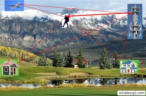
Figure 1: Multi-path components arriving at the Rx
In Figure 1, the direct path to the hiker is shown by the bold line. Assume that the second path arrives after a delay of $1 \mu s$ of the direct path (say, from the aeroplane) and the third path arrives after another $1 \mu s$, i.e., a total of $2 \mu s$ after the direct path. We will use these numbers in our examples below.
In the discussion that follows, we avoid technical terms such as delay spread, frequency-selective fading, frequency flat fading and so on. Also, we ignore the RF carrier in the subsequent discussion to highlight the important concepts relevant to the current discussion.Finally, we will consider binary modulation to avoid using the term symbols and stick to bits instead.
You can also watch the video below.
Digital Modulation
Digital modulation is concerned with mapping of the bits (1s and 0s) to a property of the signal suitable for transmission. For example, consider a rectangular pulse shape. Amplitude modulation maps 0s and 1s to $\pm 1$ as
$$0 \rightarrow -1 $$
$$1 \rightarrow +1$$
that correspondingly alters the amplitude of the rectangular pulse shape, as shown in Figure 2 below.

Figure 2: Amplitude modulation
Here, a bit stream 01001010 is mapped to the sequence -1,+1,-1,-1,+1,-1,+1,-1. In this simple system, all the Rx has to do is compare the amplitude of the received signal level (within each bit time) to a threshold (say, 0) and decide in favor of +1 or -1 (and consequently, 1 or 0).
A Low Data Rate Signal
Suppose that the year is early 2000s and our hiker in Figure 1 only wants to check his email and/or messages (probably driven by what is available) and requires a data rate of only $100$ kbps. That translates to a bit time (also known as bit duration) of
$$1/100,000 = 10 \mu s$$
as drawn in Figure 3.
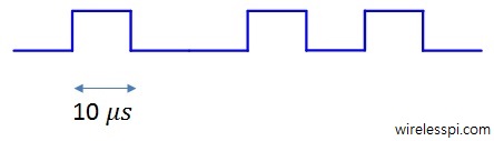
Figure 3: A low rate $100$ kbps signal with a bit duration equal to $10 \mu s$
As described above, the first and second multi-path components arrive $1 \mu s$ and $2 \mu s$ after the direct path, respectively (ignoring the carrier). This is shown in Figure 4.
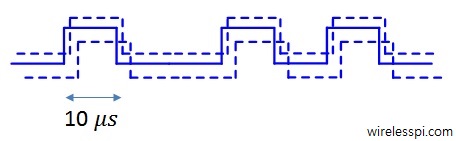
Figure 4: First and second multipath components arriving after $1$ and $2$ $\mu s$ after the direct path, respectively (carrier wave not shown)
Since nature adds the signals at the antenna, the Rx will have a summation of these three paths, effectively the same signal delayed by different amounts but with different attenuation and phase shifts of the carrier waves (not drawn in the figure). Those phase shifts depend on the path delay and the carrier frequency. Observe that $2 \mu s$ is $20 \%$ of the bit duration $10 \mu s$, an implication of which is that multi-path components will distort the Rx signal but there will not be much interference among the bits themselves. That is to say that bit 1 through its last path will interfere slightly with bit 2 to a little extent but not with any other bit farther than that.
This is a situation that can be handled without much effort in terms of computational resources. We claim that the wireless channel does not pose a significant problem to Rx processing time in this low data rate scenario. It is not necessary to understand this in the context of this article but the disadvantage here is that in case of destructive interference, there is no other way to recover except providing diversity to the Tx signal. Diversity is a signal replica in some form whether in time, frequency, space, etc.
Moving towards High Data Rate
Fast forward to a decade, say early 2010s. Escaping the fast pace of life, our hiker wants to sit on top of that peaceful mountain …. to watch YouTube videos. In fact, he considers having access to it anywhere as a basic necessity of life like water and electricity. Assume that a data rate of $10$ Mbps is needed for this purpose, which translates to a bit duration of $0.1 \mu s$ as shown in Figure 5.
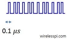
Figure 5: A high rate $10$ Mbps signal with a bit duration equal to $0.1 \mu s$
The main point is that the environment is still the same and does not care about our data rates! Multi-path components previously arriving $1$ and $2 \mu s$ after the direct path will still arrive $1$ and $2 \mu s$ after the direct path. This is illustrated in Figure 6 (again ignoring the carrier). The different path lengths will translate into different attenuations and phase shifts resulting in constructive and destructive interference throughout the signal span.
Figure 6: First and second multipath components still arrive after $1$ and $2$ $\mu s$ after the direct path, respectively (carrier wave not shown)
What does this imply for the high rate transmission? Notice that in this case, the initial bits of the transmission are interfering with many tens of bits in the future through the late arriving paths, a phenomenon known as Inter-Symbol Interference (ISI). In most cases of interest, this ISI could have been observed even extending to hundreds or even thousands of bits. We can conclude that the same harmless channel for low rate communication has become harsh for high rate communication!
A solution must be devised for this problem.
Solution – Equalizer
It turns out that a solution for this kind of problem was devised by Robert Lucky at Bell Labs in 1964: an adaptive equalizer. An equalizer is a filter that mitigates the effects of channel fading on the Rx signal and removes the Inter-Symbol Interference (ISI). Its input is the distorted waveform (sum of the original signal and its multi-path components) and the output is the clean desired bit stream as shown in Figure 7. An LMS equalizer is one such example.

Figure 7: Equalizer input is a distorted waveform and its output is a clean bit stream
Don’t think of it as a physical device. Just like everything physical got transformed into digital logic in the history of communications (leading to software defined radios), an equalizer sits as mere lines of code in a microprocessor.
An equalizer has its advantages and disadvantages. Needless to say, it considerably improves the bit error rate and consequently fundamental to making the system functional. Technically, it exploits the frequency diversity available in a broad spectrum. On the other hand, for a high rate system, it is the most demanding and resource intensive component of a conventional wireless Rx. While the exact numbers depend on the requirements and implementation, it can consume even 75% of the processing resources! In high speed communication, it is impractical to be busy processing a bit in a certain window of time while many future bits are arriving at the Rx. That will result in filling the buffer faster than being emptied.
We can conclude that a low data rate communication requires a relatively simple Rx processor while high rate communication requires a heavy duty Rx processor. That kind of processing demands high power consumption and hence not feasible for battery operated devices like our smart phones.
Can there be a technique to achieve fast communication with a simpler equalizer? The answer is yes and the technique is OFDM.
OFDM in Time Domain
In time domain, OFDM breaks one serial fast bit stream into many parallel slow bit streams.
Then, these parallel slow bit streams are multiplied with orthogonal sinusoids, where orthogonality between two sinusoids is defined with a summation over a certain time interval as
$$\sum \limits _{n=0} ^{N-1} \cos 2\pi k f_0 n \cdot \cos 2\pi k’ f_0 n = 0$$ when $k \neq k’$.
This process is illustrated in detail in Figure 8 with the help of an example:
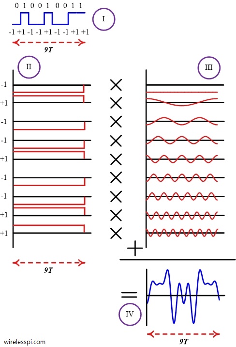
Figure 8: An OFDM example in time domain. See below for details
For a bit stream $b[k]$, the example in Figure 8 traces the following steps:
I. Assume that the bit duration is $T$ and there are 9 bits to be sent. In a high speed communication system, it will take $9T$ seconds to transmit all the bits. So we break them down to 9 parallel bit streams each with a duration of $9T$ seconds.
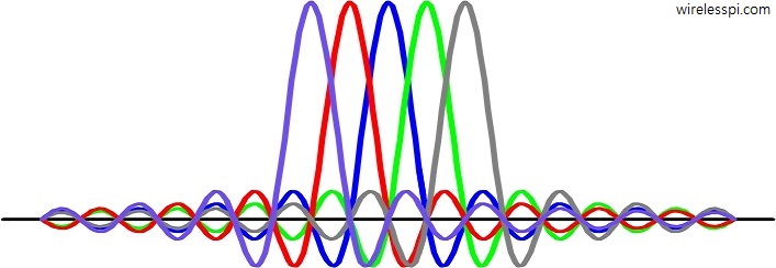
II. Assume a fundamental frequency of $f_0 = 1/9T$ with 9 samples within this duration (that will be one complete period). Then, this sinusoid will be orthogonal to 8 other sinusoids with frequencies $0f_0$, $2f_0$, $3f_0$, $\cdots$, $8f_0$. This set of 9 sinusoids is shown in Figure 8. We will call them subcarriers.
III. Next, we multiply each such sinusoid with $+1$ or $-1$ (depending on the bit) to scale their amplitude accordingly.
$$b[k]\cdot \cos 2\pi \frac{k}{9} n$$
IV. Finally, all these amplitude scaled sinusoids are added together to generate the desired signal. Notice that this composite signal has a duration of $9T$ seconds (same duration as the original bit stream) but contains the information from all 9 bits.
For a bit stream $b[k]$ mapped to a non-binary modulation scheme $X[k]$ (having I and Q components) and $N$ sinusoids (instead of 9), this sequence of steps can be carried out using the inverse Discrete Fourier Transform (iDFT) defined as
$$s[n] = \frac{1}{N} \sum \limits _{k=0} ^{N-1} X[k] e^{j2\pi \frac{k}{N}n}$$
The question is what we have achieved so far. For each such individual signal, the multi-path components arrive in not
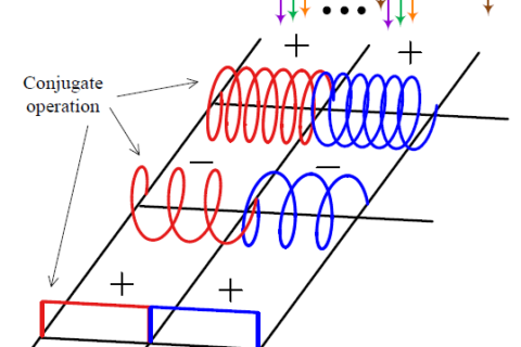
too distant future (just like a low rate stream above). The multi-path components for individually modulated subcarriers as well as for the composite signal are shown in Figure 9.
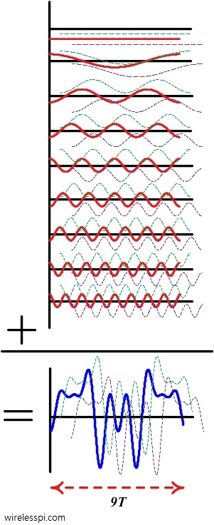
Figure 9: Multi-path components for individually modulated subcarriers as well as the composite signal. First and second path respectively shown up and down for clarity
Hence, the equalizer design is easy having less spread paths and consequently less interference with future symbols,
provided that we find a way to separate the subcarriers at the Rx. Separating these bits at the Rx is easy: we can correlate (multiply sample by sample and sum) the composite signal with just one subcarrier, say with frequency $6f_0$. Utilizing their orthogonality property, contribution from all other 8 subcarriers will cancel out to zero, while the contribution from the subcarrier with that frequency $6f_0$ will pop out, scaled in amplitude by our modulation signal. The same procedure can be repeated for all other subcarriers.
Essentially, this is an operation of Discrete Fourier Transform (DFT) as
$$X[k] = \sum \limits _{n=0} ^{N-1} s[n] e^{-j2\pi \frac{k}{N}n}$$
which, for each $k$, will generate our modulate data.
OFDM in Frequency Domain
The wireless channel shown in Figure 1 has an impulse response derived from the contribution of each multi-path component. It also has a frequency response, assume that it has a shape as in Figure 10.
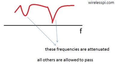
Figure 10: Frequency response of the wireless channel
With respect to frequency domain, the signal at the Rx is a product of the spectra of the Tx signal and the wireless channel. Thus, the channel will allow some frequencies to pass through unharmed while suppressing some others. We will come to this point later.
Now remember that time and frequency have inverse relationship. A signal wide in time domain has a narrow frequency span and vice versa. Although this relationship can be derived, we can just look into the Fourier transform of a rectangular signal: a sinc signal. The wider the rectangle, the earlier the sinc’s first zero-crossing is. Therefore, a low rate signal being wide in time domain has a narrow spectral representation. On the other hand, a fast rate signal exhibiting rapid changes in time has a wide spectrum. While random data generates a random signal that in turn is defined in terms of power spectral density, the underlying concept is still true and is drawn in Figure 11.
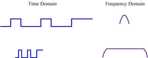
Figure 11: Spectral contents of a signal depend on its variations in time
As mentioned earlier, their interaction with the channel is through multiplication of spectral responses. The low data rate signal needs less manipulation by the Rx to get the original data back. Essentially for this kind of signal, as seen in Figure 12, the channel acts just as a single multiplier that can be equalized through estimating that number (known as channel estimation) and dividing the Rx signal by that number. So the equalization reduces to a single division operation.
There can be a question of how to recover when the narrowband signal appears within a deep channel fade. In that case, nothing but diversity (a signal replica in some form whether in time, frequency, space, etc.) can recover the signal which is out of scope of this article.
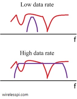
Figure 12: Signal bandwidth plays a central role in determining how it is treated by the channel
On the other hand, a high data rate signal needs a lot of Rx processing to equalize the channel. Figure 12 illustrates how different portions of the signal spectrum are treated differently by the channel and a complex algorithm needs to be implemented for signal recovery. There is an advantage in this situation in the form of available ‘frequency diversity’ which prevents the whole signal spectrum to go down in a deep fade (as opposed to low data rate case above). Equalizer inherently exploits that same frequency diversity which is outside the scope of this article. However, remember that we cannot afford a computationally expensive equalizer and instead need a simpler one.
To solve this problem, what OFDM does in frequency domain is fairly simple. It just segments the available bandwidth into many parallel almost flat channels through utilizing those sinusoidal subcarriers. Hence, equalization for each narrow slice requires just a single division operation, rendering the computational load of the equalizer to a total of $N$ divisions. This is illustrated in Figure 13.
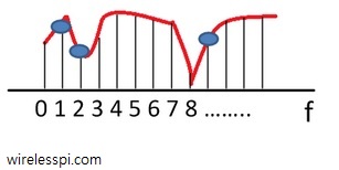
Figure 13: In frequency domain, OFDM slices the spectrum through using the subcarriers; now each spectral segment can be processed individually
The situation is very similar to processing a bread. Each time a person wanted to eat bread, they had to take a knife and cut a piece of bread for themselves. Then came sliced bread in 1928 that changed everything. Processing each individual slice got much easier; you could put jam, butter or cheese on different slices. See Figure 14 below.

Figure 14: Just like a whole bread needs to be sliced for eating convenience, OFDM slices the spectrum for communication convenience
It was difficult to process a whole bread before that invention. Similarly, it is difficult to process the collective spectrum for communication purposes. By slicing the spectrum, OFDM not only made it easier to equalize the wireless channel but also made it possible to send different modulation signals on different subcarriers (e.g., subcarriers experiencing ‘good’ channel can be used to transmit a higher-order modulation signal that translates into more bits within the same time). On a lighter note, now we have a formal proof that OFDM is the best thing since sliced bread.
Summary
- In time domain, OFDM converts one serial fast bit stream into many parallel slow bit streams.
- In frequency domain, OFDM segments one wide spectrum into many narrow spectra.
Concluding Remarks
There are a few remarks for readers who might have the following questions in their minds.
1. A question that can be asked at this stage is that why OFDM figure in articles and textbooks looks different than Figure 13. The reason is that a sinusoidal subcarrier has a spectral shape that is a single impulse. However, when that sinusoid is limited in time, it is equivalent to multiplying it with a rectangular signal. Since Fourier transform of a rectangle is a sinc signal, and multiplication in time domain is convolution in frequency domain, we get a sinc signal for each subcarrier – shifted in frequency according to the frequency of that subcarrier. The actual OFDM spectrum obtained through the DFT operation, though still sliced, is drawn in the figure below.
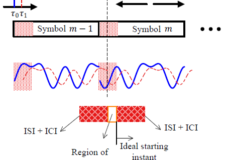
2. How does OFDM eliminate the ISI arising from the neighboring symbols (like the multi-path in above figures)? For this purpose, a gap can be left between two subsequent symbols so that multi-path components of the first do not interfere with the second. However, for numerous reasons, something known as a cyclic prefix is actually used.
3. Like single-carrier systems, windowing can also be applied to an OFDM signal, as explained here.
4. See a complete list of advantages and disadvantages of an OFDM system here.
5. Due to its particular waveform structure, the impact of timing errors is not as as much pronounced in OFDM as in single-carrier systems. A Schmidl and Cox synchronization technique is usually applied for timing synchronization in OFDM systems
6. In 5G systems, an OFDM waveform is adopted for both uplink and downlink operation. Nevertheless, a variant of OFDM, known as DFT-precoded OFDM, is also available for uplink transmission.
This is a short summary of how OFDM works. For a reader interested in gaining more design knowledge (including synchronization and equalization solutions), see my book on wireless communications or the SDR course.
Thanks for putting it simply. Now I have some basic understanding of OFDM. The article can be converted to a 5-minute video
I am glad that you liked it. Thanks for the video suggestion. I have done it in my course on wireless communications.
This is good even for non-beginners. It is like seeing the scaffolding around a structure to understand how it was built, and why it has the final shape.
Nice analogy! Thanks for the appreciation.
A very good and intuitive guide for OFDM. Thanks.
Any discussion on OFDM is not complete without a discussion of Cyclic Prefix. Great article nonetheless.
You’re right. I am going to write about it in a separate article soon. The nature of the blog implies that everything about a certain topic cannot be covered in a single post.
Nicely written – easy to understand and absorb broader picture. Thanks Qasim.
Thanks Dinuka
Very nice article sir…I have a doubt. How much is the frequency spacing and how long does the OFDM symbol lasts (in the above article OFDM symbol s[n] n will vary from … to … ??? )
Thanks. The frequency spacing is 1/T where T is one symbol time. The length of the OFDM symbol is given by the symbol time T plus the length of they cyclic prefix T_cp.
Fantastic article that I have been returning to over the years!
Thanks for your kind words 🙂