Minimum Shift Keying (MSK) is one of the most spectrally efficient modulation schemes available. Due to its constant envelope, it is resilient to non-linear distortion and was therefore chosen as the modulation technique for the GSM cell phone standard.
MSK is a special case of Continuous-Phase Frequency Shift Keying (CPFSK) which is a special case of a general class of modulation schemes known as Continuous-Phase Modulation (CPM). It is worth noting that CPM (and hence CPFSK) is a non-linear modulation and hence by extension MSK is a non-linear modulation as well. Nevertheless, it can also be cast as a linear modulation scheme, namely Offset Quadrature Phase Shift Keying (OQPSK), which is a special case of Phase Shift Keying (PSK). As a borderline case, these relationships are illustrated in the figure below.

Figure 1: MSK as a special case of both non-linear and linear modulation schemes
At this point, you would be thinking about the following question: How can a modulation be both non-linear and linear? As we see later in this tutorial, originally MSK is a non-linear modulation but a certain depiction of its actual digital symbols known as pseudo-symbols turns it into an OQPSK representation.
Modulation is a simple topic to understand but owing to the above description, MSK can sometimes be an intimidating concept. Here, our purpose is to present it in an uncomplicated manner by building it through the fundamentals.
The starting point is one of the simplest digital modulations possible: FSK.
Binary Frequency Shift Keying (BFSK)
In Frequency Shift Keying (FSK), digital information is transmitted by changing the frequency of a carrier signal. Naturally, Binary FSK (BFSK) is the simplest form of FSK where the two bits 0 and 1 correspond to two distinct carrier frequencies $F_0$ and $F_1$ to be sent over the air. The bits can be translated into symbols through the relations
$$0 \quad \rightarrow \quad -1$$
$$1 \quad \rightarrow \quad +1$$
This enables us to write the frequencies $F_i$ with $i ~ \epsilon ~ \{0,1\}$ as
$$F_i = F_c + (-1)^{i+1} \cdot \Delta_F = F_c \pm \Delta_F$$
where $F_c$ is the nominal carrier frequency and $\Delta_F$ is the peak frequency deviation from this carrier frequency. Consequently,
\begin{equation*}s(t) = A \cos 2\pi F_i t = A \cos\Big[2\pi \big\{F_c \pm \Delta_F\big\} t\Big]\quad —- \quad \text{Eq (1)}\end{equation*}
where $$0\le t \le T_b$$
Figure 2 below displays a BFSK waveform for a random stream of data at a rate of $R_b = 1/T_b$. Note that we are not distinguishing between a bit period and a symbol period because both are the same for a binary modulation technique.
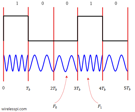
Figure 2: A Binary Frequency Shift Keying (BFSK) waveform
As is evident from Figure 2 above, the phase transitions at the boundaries of bit transitions are — in general — discontinuous. In case you are interested, an FSK signal can be demodulated through several methods such as quadrature demod, correlators or matched filtering, a Phase Locked Loop (PLL), bandpass filters, limiter discriminator, and so on.
Minimum Frequency Spacing
Although any two distinct frequencies $F_0$ and $F_1$ can be used for communication purpose, it greatly helps in receiver design if the two distinct signals are orthogonal to each other, i.e.,
$$\int \limits _0 ^{T_b} s_1(t) s_0(t) ~dt = 0$$
A question that arises at this stage is the following: how close can the two frequencies $F_0$ and $F_1$ be? Or in other words, what is the smallest possible value of $\Delta_F$? The reason for asking this question is spectral efficiency. The closer the two frequencies, the more the number of channels available for other users in the same spectrum.
For a BFSK case,
\begin{equation*}
\int \limits _0 ^{T_b} \cos 2 \pi F_1 t \cos 2 \pi F_0 t ~dt = 0\end{equation*}
or
\begin{align*}
\int \limits _0 ^{T_b} \cos 2 \pi (F_1 + F_0 )t ~ dt + \int \limits _0 ^{T_b} \cos 2 \pi (F_1 – F_0 )t ~ dt &= 0 \\
\frac{\sin 2\pi (F_1+F_0)t}{2\pi (F_1+F_0)}\bigg |_{0}^{T_b} + \frac{\sin 2\pi (F_1-F_0)t}{2\pi (F_1-F_0)}\bigg|_{0}^{T_b}&= 0 \\
\frac{\sin 2\pi (F_1+F_0)T_b}{2\pi (F_1+F_0)} + \frac{\sin 2\pi (F_1-F_0)T_b}{2\pi (F_1-F_0)}&= 0
\end{align*}
Since $F_1+F_0 = 2F_c ≫ 1$ while $-1 \le \sin x \le 1$, the first term goes to zero and we can write
\begin{equation*}
\sin 2\pi (F_1-F_0) T_b = 0
\end{equation*}
which is true for (remember $\sin k\pi = 0$ for integer $k$)
$$2\pi (F_1-F_0) T_b = k\pi$$
From here, the orthogonality condition can be concluded as
$$F_1-F_0 = \frac{k}{2T_b}$$
This also yields the minimum frequency separation for $k=1$.
$$F_1-F_0 = \frac{1}{2T_b} = \frac{R_b}{2}$$
for orthogonal signaling. Thus, the peak frequency deviation $\Delta_F$ can be computed as
$$\Delta_F = \frac{F_1-F_0}{2} = \frac{1}{4T_b} = \frac{R_b}{4}$$
MSK as Continuous-Phase FSK
From the above information, a BFSK signal with minimum tone spacing can be constructed by replacing $\Delta_F$ by $R_b/4$ in Eq (1) as
\begin{align*}s(t) &= A \cos \Big[2\pi \big\{F_c \pm \frac{R_b}{4}\big\} t\Big], \\
&= A \cos \Big[2\pi F_c t \pm 2\pi\frac{R_b}{4} t\Big], \quad 0\le t \le T_b
\end{align*}
This is a CP-BFSK signal with minimum tone spacing defined over a single bit interval $0 \le t \le T_b$. There are two more steps to construct an actual MSK waveform.
- In a real communication system, the signal is constructed by transmitting a sequence of bits $b_n$ in succession, where $n$ is the bit index. As we have seen earlier, bits $b_n ~\epsilon~ \{0,1\}$ are converted to symbols $a_n$.
$$a_n ~\epsilon~ \{-1,+1\}$$
Then, in the interval $nT_b \le t \le (n+1)T_b$, the above signal can be written as
\begin{align*}
s(t) &= A \cos \Big[2\pi F_c t + 2\pi\frac{a_n R_b}{4} (t-nT_b)\Big], \quad nT_b \le t \le (n+1)T_b
\end{align*} where $n$ is the bit index within a long bit stream and the second term indicates the underlying baseband message. - Observe in the above equation that the phase continuity is not necessarily maintained from one symbol to the next. To ensure phase continuity, we must add a phase component for each symbol as
\begin{align*}s(t) &= A \cos \Big[2\pi F_c t + 2\pi\frac{a_n R_b}{4} (t-nT_b) + \theta_n\Big] \\ & \qquad \qquad nT_b \le t \le (n+1)T_b \quad —- \quad \text{Eq (2)}\end{align*}
For this purpose, the phase at both sides of $t=(n+1)T_b$ must be equal, as illustrated in Figure 3.
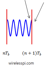
Figure 3: Phase on both sides of $t=(n+1)T_b$ must be equal to maintain continuity
Thus, at the instant $t=(n+1)T_b$, the following equation must be satisfied.
\begin{align*}
2\pi \frac{a_n R_b}{4} (t-nT_b) + \theta_n \bigg |_{t=(n+1)T_b} &= 2\pi \frac{a_{n+1} R_b}{4} (t-(n+1)T_b) + \theta_{n+1} \bigg |_{t=(n+1)T_b}
\end{align*}
which can be written as $$\theta_{n+1} = \theta_{n} + a_n \frac{\pi}{2}$$
Another way to write the above recursive relation is
\begin{equation*}\boxed{\theta_{n} = \theta_{n-1} + a_{n-1} \frac{\pi}{2}}\quad —- \quad \text{Eq (3)}\end{equation*}
Assume that $\theta_0 = 0$. Then,
$$\theta_1 = a_0 \frac{\pi}{2}$$
$$\theta_2 = \theta_1 + a_1 \frac{\pi}{2} = \frac{\pi}{2} (a_0+a_1)$$
In general,
$$\theta_n = \frac{\pi}{2} \sum \limits_{i=0}^{n-1} a_i \quad —- \quad \text{Eq (4)}$$
When the phase follows this rule during each bit/symbol interval, the phase continuity is ensured and the resulting waveform is shown for an example sequence in Figure 4.
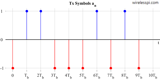
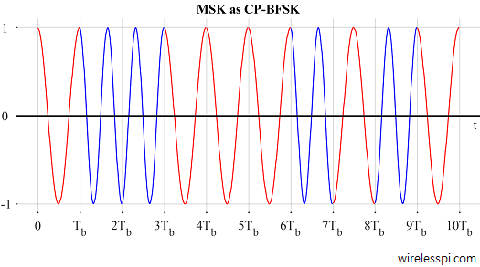
Figure 4: MSK as Continuous-Phase Binary FSK
Notice how Figure 4 is different than Figure 2 in phase continuity.Below, we plot $\theta_n$ as a function of time in Figure 5 to see how it evolves. One can observe that it indeed changes values in steps of $\pi/2$ depending on the last data bit.
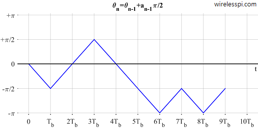
Figure 5: $\theta_n$ evolving with time
MSK as Offset QPSK
First, write Eq (2) assuming $A=1$ as \begin{align*}s(t) &= \cos \Big[2\pi F_c t + 2\pi \frac{a_n R_b}{4} (t-nT_b) + \theta_n\Big] \\ &= \cos \Big[2\pi F_c t + 2\pi \frac{a_n R_b}{4} t \underbrace{-na_n \frac{\pi}{2} + \theta_n}_{\Theta_n}\Big]\quad —- \quad \text{Eq (5)} \end{align*} Using Eq (3), we can further manipulate $\Theta_n$ as \begin{align*} \Theta_n &= \theta_n – na_n \frac{\pi}{2} \\ &= \theta_{n-1} + a_{n-1}\frac{\pi}{2} – na_n \frac{\pi}{2} \\ &= \theta_{n-1} + a_{n-1}\Big(+1-n+n\Big)\frac{\pi}{2} – na_n \frac{\pi}{2} \\ &= \theta_{n-1} – (n-1)a_{n-1}\frac{\pi}{2} + n \frac{\pi}{2} \Big(a_{n-1} – a_n\Big)\\ &= \Theta_{n-1} + n \frac{\pi}{2} \Big(a_{n-1} – a_n\Big)\quad —- \quad \text{Eq (6)} \end{align*} Notice that $\Theta_{n} = \Theta_{n-1}$ when
- $a_n = a_{n-1}$ because the second term in Eq (6) becomes zero.
- $n$ is even because the second term in Eq (6) is a multiple of $2\pi$ (remember that $a_{n-1}-a_n$ is $\pm 2$ when not zero).
We conclude that $\Theta_n$ can only change when $a_n \neq a_{n-1}$ and $n$ is odd. In that case, it will always change by an odd multiple of $\pm \pi$. In summary, considering modulo-$2\pi$ operations,
$$\Theta_n = \begin{cases}
\Theta_{n-1}\pm \pi & a_n \neq a_{n-1}, n~\text{odd} \\ \Theta_{n-1} & \text{otherwise} \end{cases}\quad —- \quad \text{Eq (7)}$$
Next, we use the following identities \begin{align*} \cos (\alpha\pm \beta) &= \cos \alpha\cos \beta \mp \sin \alpha \sin \beta \\ \sin (\alpha\pm \beta) &= \sin \alpha\cos \beta \pm \cos \alpha \sin \beta \\ \cos (-\alpha) &= \cos \alpha \\ \sin (-\alpha) &= – \sin \alpha \end{align*} to open Eq (5). \begin{align*} s(t) &= \cos \Big[2\pi F_c t + 2\pi \frac{a_n R_b}{4} t + \Theta_n \Big] \\ &= \cos 2\pi F_c t \cdot \underbrace{\cos \Big(2\pi \frac{a_nR_b}{4}t + \Theta_n\Big)}_{\text{Term 1}} – \\ &\qquad \qquad \qquad \sin 2\pi F_c t\cdot \underbrace{\sin \Big(2\pi \frac{a_nR_b}{4}t + \Theta_n\Big)}_{\text{Term 2}} \end{align*} Now we process both terms one by one. \begin{align*} \text{Term 1} &= \cos \Big(2\pi \frac{a_nR_b}{4}t + \Theta_n \Big) \\ &= \cos \Big(2\pi \frac{a_nR_b}{4}t\Big) \cos \Theta_n – \sin \Big(2\pi \frac{a_nR_b}{4}t\Big) \sin \Theta_n \\ &= \cos \Big( 2\pi \frac{a_nR_b}{4}t\Big) \cos \Theta_n = d_{I,n} \cos 2\pi \frac{R_b}{4}t\\ \end{align*} because $\Theta_0 = 0$ implies $\sin \Theta_n = 0$, see Eq (7). Furthermore, $a_n ~\epsilon~\{-1,+1\}$ and $\cos (\pm \alpha) = \cos \alpha$. We have also defined $$ d_{I,n} = \cos \Theta_n$$ Similarly, Term 2 can be expanded as \begin{align*} \text{Term 2} &= \sin \Big(2\pi \frac{a_nR_b}{4}t + \Theta_n \Big) \\ &= \sin \Big(2\pi \frac{a_nR_b}{4}t \Big) \cos \Theta_n + \cos\Big(2\pi \frac{a_nR_b}{4}t\Big) \sin \Theta_n \\ &= \cos \Theta_n \cdot a_n \sin 2\pi \frac{R_b}{4}t = d_{Q,n} \sin 2\pi \frac{R_b}{4}t \end{align*} since $\sin \Theta_n = 0$ as before and $\sin (-\alpha) = – \sin (\alpha)$. Here, we have defined $d_{Q,n}$ as $$d_{Q,n} = a_n \cdot \cos \Theta_n = a_n \cdot d_{I,n}$$ Finally, plugging both Term 1 and 2 into $s(t)$ for the $n$-th bit period, $$s(t) = d_{I,n} \cos 2\pi \frac{R_b}{4}t \cdot \cos 2\pi F_c t – d_{Q,n} \sin 2\pi \frac{R_b}{4}t \cdot \sin 2\pi F_c t$$ Using the identity $\cos \alpha = \sin (\alpha + \pi/2)$, the above equation can be revised as \begin{align*} s(t) &= d_{I,n} \sin \Big(2\pi \frac{R_b}{4}t + \frac{\pi}{2} \Big) \cdot \cos 2\pi F_c t – d_{Q,n} \sin 2\pi \frac{R_b}{4}t \cdot \sin 2\pi F_c t \\ &= d_{I,n} \sin \Big(2\pi \frac{R_b}{4}(t+T_b)\Big) \cdot \cos 2\pi F_c t – \\&\qquad \qquad \qquad d_{Q,n} \sin 2\pi \frac{R_b}{4}t \cdot \sin 2\pi F_c t\quad —- \quad \text{Eq (8)}\\ =& d_{I,n} p(t+\frac{1}{2}2T_b) \cdot \cos 2\pi F_c t – d_{Q,n} p(t) \cdot \sin 2\pi F_c t \end{align*} where $p(t)$ is a half-sinusoidal pulse shape of period $4T_b$.
$$p(t) = \sin \Big( 2\pi\frac{R_b}{4}t \Big)$$
The above expression resembles an OQPSK waveform for bit $n$ if the bit rate for $d_{I,n}$ and $d_{Q,n}$ is $R_b/2$ or bit period is $2T_b$, since the time offset in the $\sin$ term must be half the bit period for OQPSK. So we have to check if $d_{I,n}$ and $d_{Q,n}$ change values every other symbol.
From the definition, $d_{I,n} = \cos \Theta_n$ and Eq (7) tells that $\Theta_n$ can only change values for odd $n$. Hence, $d_{I,n}$ is indeed an $R_b/2$ rate stream.
On the other hand, $d_{Q,n}=a_n \cdot d_{I,n}$. Again, Eq (7) says that $d_{I,n}$ can only change when $a_n$ changes but that means that $a_n \cdot d_{I,n}$ stays the same. Therefore, $d_{Q,n}$ can only change for even $n$ and when $a_n$ changes values. Consequently, $d_{Q,n}$ is also an $R_b/2$ rate stream.
Since $d_{I,n}$ changes values for odd $n$ while $d_{Q,n}$ does the same for even $n$, $d_{Q,n}$ is offset with respect to $d_{I,n}$ by $T_b$ seconds, the same amount as $\cos 2\pi \frac{R_b}{4}t$ in Eq (8). Summing up everything so far, MSK can indeed be represented as an OQPSK waveform. The data rate is the same as in CP-BFSK format since two bits are being transmitted in two bit periods here as well.
This representation is illustrated in Figure 6.
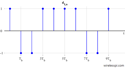
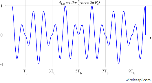
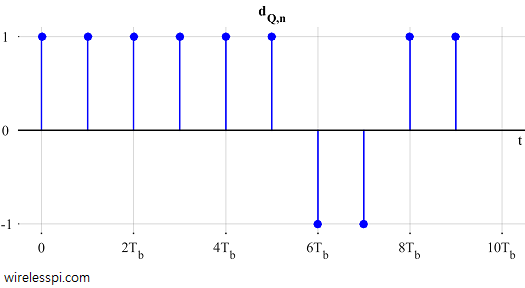
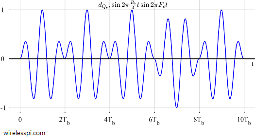
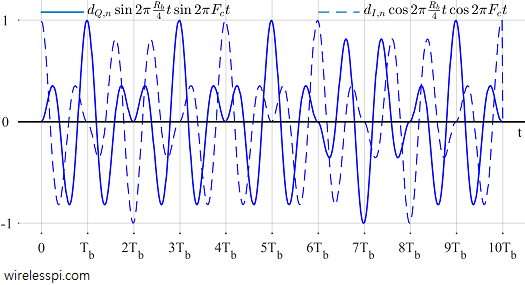
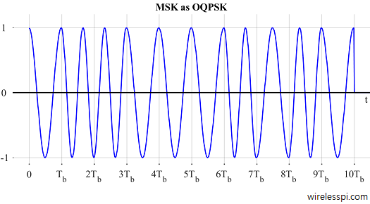
Figure 6: MSK as Offset QPSK
Compare Figure 6 with Figure 4. I did not choose separate blue and red colors in this figure so as not to confuse $d_n$s with $a_n$s (that can raise a misunderstanding that $d_{I,n}$ is odd $a_n$s and $d_{Q,n}$ is even $a_n$, which is not correct).
Observe from Figure 6 that $d_{I,n}$ is changing values every two $T_b$s at odd multiples of $T_b$, while $d_{Q,n}$ is changing values every two $T_b$s at even multiples of $T_b$. Due to this offset behavior, at every $T_b$, either $I$ or $Q$ waveform is zero at $t=T_b$ while the other reaches its maximum value. This is how phase remains continuous during symbol transitions.
Figure 7 draws $\Theta_n$ as a supplement to above findings.
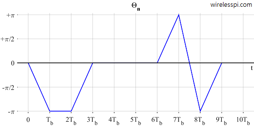
Figure 7: $\Theta_n$ evolving with time
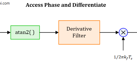
On a final note, observe from some equations (e.g., (2) and (5)) that the continuous phase has two parts, one of which arises due to the delay of the $n$-th symbol. This information can be used to refine a phase estimate.
We are also clear now why MSK can act both like a linear and a non-linear modulation. In reality, MSK is a non-linear modulation scheme (see Eq(2)) for $a_n$. Pseudo-symbols $d_n$ themselves are non-linear functions of information bits. So it is only from $d_n$ viewpoint that MSK can be seen as a linear modulation scheme.
A Generalization: From MSK to Continuous-Phase FSK (CP-FSK)
After understanding MSK, it can be expanded into a general modulation scheme known as Continuous-Phase Frequency Shift Keying (CP-FSK). As we see in the next section, CP-FSK is a special case of Continuous-Phase Modulation (CPM), which is a class of non-linear digital modulation schemes in which the phase of the signal is constrained to be continuous from one symbol to the next. As with MSK, the most attractive feature of such a signal is that it has a constant envelope as a result of the amplitude being independent of the modulating information. Consequently, a CPM signal can be amplified without distortion by a non-linear amplifier operating near the saturation point allowing low cost and more efficiency as compared to a linear amplifier.
Usually CP-FSK (and hence CPM) is not a straightforward concept to master. However, starting from MSK, its basics can easily be understood by building on the same expressions. For this purpose,
- Remember that $\Delta_F = R_b/4$.
- Modulation symbols can carry more than 1 information bit. For example, 00, 01, 11 and 10 can be sent through four symbols $a_n$ $\epsilon$ $\{-3,-1,+1+3\}$. In general, $a_n$ is a sequence from the alphabet $\{\pm 1, \pm 3, \cdots,\pm (M-1)\}$. Thus, we call $a_n$ as symbols and replace $T_b$ with $T_M$ (a symbol time) from here onwards. Symbol rate $R_M$ is then $1/T_M$.
Now let us start with rewriting Eq (2) and Eq (4) and then substituting the former into the latter.
$$\theta_n = \frac{\pi}{2} \sum \limits_{i=0}^{n-1} a_i$$
\begin{align*}
s(t) &= A \cos \Big[2\pi F_c t + 2\pi\frac{a_n R_M}{4} (t-nT_M) + \theta_n\Big] \\
&=A \cos \Big[2\pi F_c t + 2\pi \frac{1}{2}\cdot \frac{t-nT_M}{2T_M}a_n + \frac{\pi}{2} \sum \limits_{i=0}^{n-1} a_i\Big] \\
&= A \cos \Big[2\pi F_c t + 2\pi h a_n \cdot q(t-nT_M) + \pi h \sum \limits_{i=0}^{n-1} a_i\Big]
\end{align*}
where we have defined the following terms.
\begin{align*}
h &= \frac{1}{2} \\
q(t) &= \begin{cases}
0 & t \le 0 \\
\frac{t}{2T_M} & 0 \le t \le T_M \\
\frac{1}{2} & t \ge T_M
\end{cases}
\end{align*}
It turns out that $h$ is a general concept known as
modulation index, which in case of MSK is equal to $1/2$. In general, $h$ is defined as
$$h = 2 \frac{\Delta_F}{R_M}$$
which describes the peak frequency deviation in terms of a percentage of the symbol rate. With the definition of $h$, we can write
$$s(t) = A \cos \Big[2\pi F_c t + 2\pi h \Big( a_n q(t-nT_M)+ \frac{1}{2} \sum \limits_{i=0}^{n-1} a_i\Big)\Big]$$
The above equation is true for the interval $nT_M \le t \le (n+1)T_M$. Considering from its definition that $q(t)$ is $1/2$ after a symbol interval, we can also write $s(t)$ as
\begin{align*}s(t) &= A \cos \Big[2\pi F_c t + 2\pi h \sum \limits _{i=0}^{n} a_i q(t – iT_M) \Big]\quad —- \quad \text{Eq (9)}\\
&= A \cos \Big[2\pi F_c t + 2\pi h \int _{-\infty}^{t} \Big( \sum \limits _{i=0}^n a_i g(u – iT_M)\Big) du \Big]
\end{align*}
where $g(t)$ is defined as the derivative of $q(t)$ as
$$q(t) = \int \limits _{0}^{t} g(u) du$$
Notice that in the present case with $q(t)$ defined as above, its derivative $g(t)$ is a rectangular pulse shape. Consequently, $\sum \limits _i a_i g(u – iT_M)$ is the standard baseband Pulse Amplitude Modulated (PAM) waveform with rectangular pulse shape and this is how its discontinuities are transformed into a continuous-phase signal.
It is refreshing to conclude that the starting point for a continuous-phase modulated signal is a standard pulse amplitude waveform, in which the discontinuities are smoothed out by the integral operation.
More Generalization: From Continuous-Phase FSK (CP-FSK) to Continuous-Phase Modulation (CPM)
Now referring to Eq (9), the expression for a CPM signal can be written as
$$s(t) = A \cos \Big[2\pi F_c t + 2\pi \sum \limits _{i=0}^{n} h_i \cdot a_i q(t – iT_M) \Big]\qquad nT \le t \le (n+1)T$$
Here, $h_i$ is a sequence of modulation indices: a ratio of two relatively prime integers.
$$h = \frac{k}{p}$$
This is the case of multi-h CPM. When all $h_i=h$, the modulation index is the same for all symbols. This is the category we saw in CP-FSK and MSK above.
Finally, $q(t)$ is a waveform shape known as the phase response of the modulator which is normalized as
$$q(t) = \begin{cases}
0 & t \le 0 \\ \frac{t}{2T} & 0 \le t \le LT \\
\frac{1}{2} & t \ge LT
\end{cases}$$
where $L$ is the length of a pulse $g(t)$ in symbols. Since angular frequency is the rate of change of phase, this $g(t)$ is the derivative of $q(t)$ and known as the frequency response of the modulator.
$$g(t) = \frac{dq(t)}{dt}$$
For any pulse shape $g(t)$, $L=1$ results in full response CPM, while the other case $L>1$ is the partial response CPM. Commonly used pulse shapes are rectangular (as used in the case of MSK), raised cosine and Gaussian.
We can see that CPM is in fact a very large class of modulation schemes owing to different pulse shapes $g(t)$, modulation indices $h_i$ and the modulation alphabet size $M$. That is both a blessing and a curse: blessing due to the remarkable variety of signals as its offsprings all yielding excellent spectral and power efficiencies, and curse due to the high receiver complexity. By virtue of Moore’s law, this is becoming less of an issue — thanks to powerful baseband processors in the modern age.
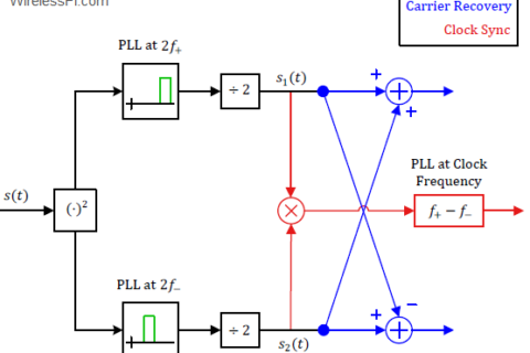
Finally, the following article describes how to acquire carrier and clock synchronization in MSK demodulators.
References
[1] Mengali and D’Andrea, Synchronization Techniques for Digital Receivers, 1997.
[2] John Proakis, Digital Communications, 4th ed, 2001.
Hello. I read your article, Ihave some questions.
1)There are a lot of sources, e.g. “http://www.dsplog.com/2009/06/16/msk-transmitter-receiver/”, “https://en.wikipedia.org/wiki/Minimum-shift_keying”,the article “Minimum shift keying: A spectrally efficient modulation Subbarayan Pasupathy, IEEE Communications Magazine, July 1979” where the coefficients Di,n and Dq,n are suggested to be the odd and even bits of the input bit stream An. You told that it is incorrect. Why?
Thanks in advance. Your site is very interesting.
Thanks for your appreciation. You can have even and odd input bit streams to generate a half-sinusoidal shaped O-QPSK waveform. However, in that case, the 0s and 1s that generate two different carrier frequencies will not be directly coming from the input, but a function of the input bits. Hope that clarifies the question.
Hi Qasim
Thanks for the fantastic tutorials.
Could you help me understand Figure 4 in your MSK tutorial. In the first bit period (0 to Tb), the signal seems to complete a full cycle, so the phase remains zero (both at t=0 and t=Tb). In the next bit period (Tb to 2Tb), the output signal goes through 1.5 cycles, so the phase must have increased by 180 deg. But Figure 5 shows phase changing from 0 to -pi/2 in 1st bit period and from -pi/2 to 0 in the 2nd period. Could you help me please.
Many thanks.
anon
Hi anon.
Great question. When you say that the phase goes from 0 to 180 etc, you are talking about the actual signal, i.e., a single CW that is changing its phase with time.
However, if you look at the equation right after the heading ‘MSK as continuous-phase FSK’, there are two different CWs, one at frequency Fc+Rb/4 and the other at Fc-Rb/4. The phase I’m talking about is introduced in Eq (2) which is the phase at time $n$ **for each bit** represented by its own CW. It only changes at bit intervals and only can take certain values (as described in the article).
Hi Qasim,
Maritime AIS has been based on GMSK. The VDES follow-on also makes use of pi/4 QPSK. Are there reasons for this particular sequence, GMSK -> pi/4 QPSK? MSK and 0-QPSK appear in the diagrams, so thought I would ask:)
Cheers, Noah
For power amplifier efficiency, modulation schemes such as GMSK having a constant envelope and pi/4 QPSK having an envelope that does not pass through zeroes are desirable for communication systems implemented on mobile platforms. This, however, is not the reason for the sequence you mentioned above : ) MSK just by design can be represented as half-sinusoidal shaped O-QPSK.
Hi Qasim,
Excellent explanation on MSK , I cleared many of my doubts in MSK , but in figure 7 phi(n) vs time ,at 8th Tb interval phi got changed from +pi to -pi. How it jumps from +pi to -pi , as per my understanding of equation 7 phi(n) = phi(n-1) when n is even ,so +pi should retain as +pi at 8th symbol interval. So please clarify my doubt.
Oh, thanks for pointing this out. +pi and -pi are the same phases (move 180 degrees from 0 either anticlockwise or clockwise and you will reach the same angle). It’s just that each programming language has its own way of handling floating point numbers as well as computing arctangent routines, which result in +pi sometimes and -pi some other times. Hope it helps.