Most signals of our interest — wireless communication waveforms — are continuous-time as they have to travel through a real wireless channel. To process such a signal using digital signal processing techniques, the signal must be converted into a sequence of numbers. This can be done through the process of periodic sampling.
From Continuous to Discrete Time
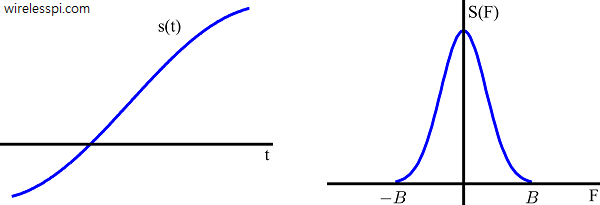
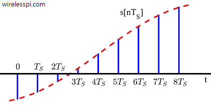
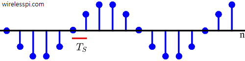
Consider a band-limited continuous-time signal $s(t)$ and its frequency domain representation $S(F)$ with bandwidth $B$, shown in the above figure. A discrete-time signal $s[n]$ can be obtained by taking samples of $s(t)$ at equal intervals of $T_S$ seconds. This process is shown in the figure below, and mathematically represented as
\begin{equation*}
s[n] = s(t)\bigg| _{t=nT_S} \quad -\infty < n < \infty
\end{equation*}
The time interval $T_S$ seconds between two successive samples is called the sampling period or sample interval, and its reciprocal $1/T_S = F_S$ is called the sample rate or sampling frequency. Sample rate $F_S$ is the most fundamental parameter encountered in digital signal processing applications.
Sampling Theorem in Frequency Domain
Let us find out what happens in frequency domain as a result of this process. Consider a continuous-time sinusoidal signal
\begin{equation*}
s(t) = A \cos (2\pi Ft + \theta)
\end{equation*}
and obtain its sampled version at a rate $F_S = 1/T_S$ samples/second.
\begin{align}
s[n] &= s(t)| _{t=nT_S} \nonumber \\
&= A \cos \left(2\pi F nT_S + \theta\right) \nonumber \\
&= A \cos \left(2\pi F \frac{n}{F_S} + \theta\right) \nonumber \\
&= A \cos \left(2 \pi \frac{F}{F_S} n + \theta\right) \label{eqIntroductionSampledSinusoid}
\end{align}
Note that $F/F_S$ above is the frequency of a discrete-time sinusoid $s[n]$. Let us sample at the same rate $F_S$ another sinusoid with continuous frequency $F + k F_S$, where $k = \pm 1, \pm 2,\cdots$.
\begin{align*}
s(t) &= A \cos \left\{2 \pi (F +kF_S) t + \theta)\right\}\nonumber \\
s[n] &= A \cos \{2 \pi (F + kF_S) nT_S + \theta\} \nonumber\\
&= A \cos \left(2 \pi \frac{F + kF_S}{F_S} n + \theta \right)\nonumber \\
&= A \cos \left(2 \pi \frac{F}{F_S} n + 2\pi kn + \theta\right) \nonumber\\
&= A \cos \left(2 \pi \frac{F}{F_S} n + \theta\right)
\end{align*}
which is exactly the same as discrete-time sinusoid in Eq \eqref{eqIntroductionSampledSinusoid}. It can be concluded that at the output of sampling process, it is impossible to distinguish between two discrete-time signals whose frequencies are $F_S$ Hz apart. So for an arbitrary frequency $F$ after sampling
\begin{align*}
F &= F + 1F_S \\
&= F – 1F_S \\
&= F + 2F_S \\
&= F – 2F_S \\
\end{align*}
and so on. It is just like saying that any two angles $360 ^\circ$ apart are all the same. For example,
\begin{align*}
30 ^\circ &= 30^\circ + 1(360^\circ) = 390 ^\circ \\
&= 30^\circ – 1(360^\circ) = -330 ^\circ \\
&= 30^\circ + 2(360^\circ) = 750 ^\circ \\
&= 30^\circ – 2(360^\circ) = -690 ^\circ
\end{align*}
Therefore, all the following frequency ranges are the same:
\begin{equation}
\begin{aligned}
&\cdots\cdot \\
-2.5F_S \quad &\rightarrow \quad -1.5F_S \\
-1.5F_S \quad &\rightarrow \quad -0.5F_S
\end{aligned}
\end{equation}
-0.5F_S \quad \rightarrow \quad +0.5F_S
\end{equation*}
\begin{align*}
0.5F_S \quad &\rightarrow \quad 1.5F_S \\
1.5F_S \quad &\rightarrow \quad 2.5F_S \\
&\cdots\cdot
\end{align*}
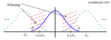
The range $-0.5F_S \rightarrow +0.5F_S$ is called the primary zone. The spectrum of the continuous-time signal $s(t)$ shown in the previous figure is now drawn in Figure below. We have indicated this zone within dotted red lines and drawn its spectral contents with solid lines while the spectral replicas with dashed lines.
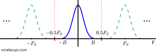
In the light of above discussion, it is evident from the figure above depicting spectral replicas that if a continuous-time signal has a bandwidth $B$ greater than $0.5F_S$, it will appear as an alias of a lower frequency within the range $-0.5F_S \le F < +0.5F_S$ and distort the signal. This is illustrated in Figure below for a signal whose bandwidth $B$ extends beyond the primary zone.
Therefore, for a signal with bandwidth B, the sampling frequency should be such that the following inequality is satisfied to prevent any distortion in the sampled signal:
\begin{equation*}
0.5F_S > B \nonumber
\end{equation*}
or written in another form
F_S > 2 B
\end{equation}
As shown above, sampling in time domain at intervals of $T_S$ creates periodicity in frequency domain with a period of $F_S = 1/T_S$. Therefore, a band-limited continuous-time signal with highest frequency (or bandwidth) $B$ Hz can be uniquely recovered from its samples provided that the sample rate $F_S \ge 2B$ samples/second.
The frequency $2B$ is called the Nyquist rate while $0.5F_S$ is called the Nyquist frequency or folding frequency. Sampling theorem is one of the two most fundamental relations in digital signal processing, the other being the relationship between continuous and discrete frequencies.
Sampling Theorem in Time Domain
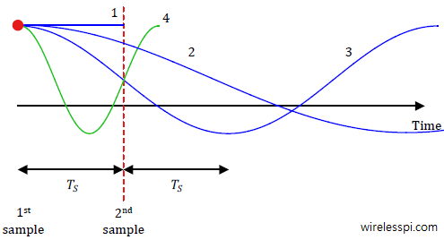
Consider a cosine wave for which two samples are taken at an interval of $T_S$. In reference to the below figure, if the frequency is zero (signal is denoted with number 1), both samples are the same and there is no confusion. For a low frequency waveform 2, again two samples can be taken that sufficiently distinguish it from waveform 1. The same can be said about waveform 3 whose period $T$ is greater than $2T_S$ in the below figure. However, notice that for waveform 4, the time period is less than $2T_S$ here, and hence it intersects the waveform 3 at the location of second sample. This makes it impossible to distinguish between waveform 3 and 4. That is how sampling theorem can be understood in time domain.

From the above figure, we can say that for a waveform with frequency $F=1/T$ and sample rate $F_S=1/T_S$,
\[
T > 2T_S, \qquad \text{or}\qquad \frac{1}{T} < \frac{1}{2T_S}
\]
The fact that a continuous frequency higher than $0.5F_S$ Hz appears similar to a frequency $F_S$ Hz apart from itself can be understood in time domain from another figure below. Observe that samples are taken at a rate such that both sinusoids pass through the same points. In fact, there are infinitely many sinusoids ($F_S$ Hz apart) which pass through the same points, and hence become indistinguishable from each other after sampling.

A natural extension is to understand the notion of time in a discrete-time setting. As long as the sampling interval or sample rate is known, one can easily determine the period or frequency of a signal. For the sinusoid of Figure below for example, the period $T$ is clearly $10$ samples, and to find it in actual seconds, sample interval $T_S$ or sample rate $F_S$ must be known.
For $T_S = 0.1$ seconds,
\begin{align*}
T &= 10 ~\frac{{samples}}{{period}}~ \cdot ~ 0.1 ~\frac{{seconds}}{{sample}} = 1~ {second}
\end{align*}
and its frequency $F = 1/T = 1$ Hz. However, for a $T_S = 0.002$ seconds, the same discrete-time sinusoid has
\begin{align*}
T &= 10 ~\frac{{samples}}{{period}}~ \cdot ~0.002 ~\frac{{seconds}}{{sample}} = 0.02~ {seconds}
\end{align*}
with frequency $F = 1/T = 50$ Hz. Interestingly, the samples of both sinusoids will be stored in memory as a sequence of numbers with no difference in discrete domain.
Aliasing – the reemergence of frequencies higher than $0.5F_S$ within the range $-0.5F_S \le F < +0.5F_S$ of primary zone - is a consequence of disobeying the sampling theorem. It may seem so but aliasing is not always bad. In fact, there are three types of aliasing:
- Harmful aliasing that distorts the signal and must be avoided for proper representation of signal in discrete domain. This is when $F_S < 2B$.
- Useful aliasing that shifts the signal spectral bands up and down for free to our desired frequency through careful system design. This is employed in systems operating at multiple clock rates.
- Harmless aliasing that is neither good nor bad for the system. This occurs, for example, during band-limited pulse shape design to avoid inter-symbol interference (ISI).
Some remarks are as follows.
- For a fixed time interval of data collection, the more samples we take, the higher the energy in the resulting discrete-time signal. This is because there will be more samples in the discrete-time signal during the same fixed interval.
- For every extra bit the ADC has, there is a 6 dB improvement in Signal to Quantization Noise Ratio.
this website is quite informative…
Thank you for the appreciation.