Transforming a discrete-time signal — whether in time or amplitude — is certainly possible, and often in interesting ways. In practice, scaling and time shifting are the two most important signal modifications encountered. Scaling changes the values of dependent variable on amplitude-axis while time shifting affects the values of independent variable on time-axis.
Below we describe addition and multiplication of two signals as well as scaling and time shifting a signal in detail.
Addition
For addition of two discrete-time signals, say $x[n]$ and $y[n]$, add the two signals sample-by-sample: $z[n] = x[n] + y[n]$ for every $n$, e.g.,
\begin{align*}
z[0] &= x[0] + y[0] \\
z[1] &= x[1] + y[1] \\
\cdots & \cdot\cdot
\end{align*}
and so on.
Multiplication
For multiplication, multiply the two signals sample-by-sample, as we did with addition: $x[n] \cdot y[n]$ for every $n$, e.g.,
\begin{align*}
z[0] &= x[0] \cdot y[0]\\
z[1] &= x[1] \cdot y[1]\\
\cdots & \cdot\cdot
\end{align*}
and so on.
Scaling
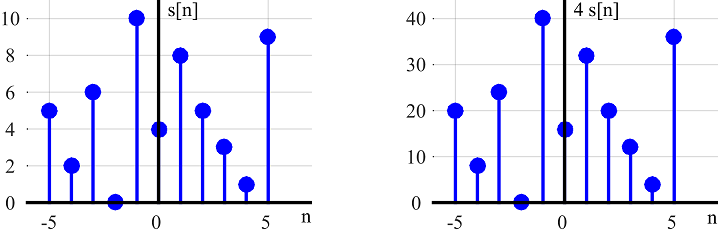
Scaling implies multiplying the signal amplitude by a constant number $\alpha$ resulting in $\alpha~s[n]$, where $\alpha$ can be positive, negative, greater than or lower than $1$. For example, Figure below shows a signal $s[n]$ scaled by 4 (compare the amplitudes of both signals on y-axis). One word of caution: The whole signal gets scaled by the same value here and hence scaling is different than sample-by-sample multiplication of two signals.
Time Shifting
A signal $s[n]$ can be shifted to the right or left by any amount $m$. There are two ways to look at time shifting a signal.
Conventional Method – Shifting the Signal
Most textbooks on discrete-time signals describe this process as follows.
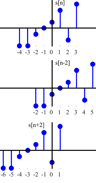
[Delay] For $s[n-m]$, the time shift results in a delay of $s[n]$ by $m$ units of time. So plot $s[n-2]$ by shifting $s[n]$ two units to the right as shown in Figure below.
[Advance] For $s[n+m]$, the time shift results in an advance of $s[n]$ by $m$ units of time. So plot $s[n+2]$ by shifting $s[n]$ two units to the left as shown in Figure below.
This is simple to remember: Write the time shift as $n-m$. Shift right for $s[n-m]$ and shift left for $s[n+m]$.
There are two problems with the approach above.
- It does not explain why we are doing what we are doing.
- A confusion might arise in the following way. The past samples of the sequence are to the left of the origin while the future samples are to the right. When we advance a signal by shifting left, a beginner might think that the future samples are on the left side. A similar argument holds for delaying a signal.
Intuitive Method – Shifting the Axis
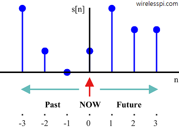
This method is based on the earliest notions of time kept by humans: past, present and future. Replacing the word present with the NOW, consider the following quote:
"Realize deeply that the present moment is all you have. Make the NOW the primary focus of your life."
In signal processing applications, NOW is the time index $0$ and we want to make it the primary focus of a signal’s life, as shown in Figure below.
Looking from this perspective,
[Delay] For $s[n-m]$, $n-m$ clearly implies traveling $m$ units in the past. So plot $s[n-2]$ by going 2 units back in time and making it the new NOW, i.e., time index 0 as shown in Figure below.
[Advance] For $s[n+m]$, $n+k$ obviously implies a future travel of $m$ units. So plot $s[n+2]$ by going 2 units towards the future and making it the new NOW, i.e., time index 0 as shown in Figure below.
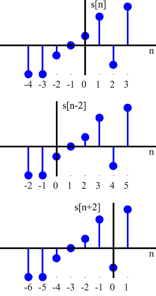
Stated in another way, just look at the time-axis itself. Keep the discrete-time signal as it is, but move 0 time index $m$ units to the left for $n-m$ and $m$ units to the right for $n+m$, as in Figure above. Notice that index 0 of $s[n+2]$ is at the same sample as index $2$ of $s[n]$, which indicates accessing a future value. Although the difference is only how to look at the process, this is a simpler and more intuitive approach. This will be very helpful when we will discuss the topic of convolution later.
Note that as far as drawing time shifted signals is concerned, we will mostly use the first approach because it saves page space by aligning the time-axis indices right on top of one another.
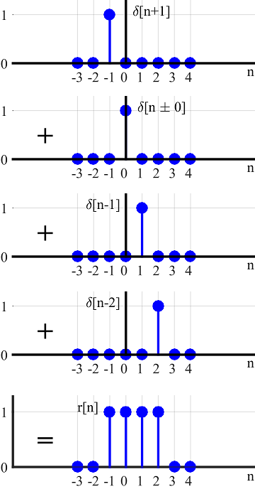
Understanding time shifting a signal makes it easy to analyze seemingly complicated equations such as
\begin{equation*}
r[n] = \sum \limits _{m=-1} ^{2} s[n-m]
\end{equation*}
which is basically addition of $s[n-m]$ for $m=-1,0,1$ and $2$. We can simply break it down to a more recognizable form by substituting values of $m$ as
\begin{equation*}
r[n] = s[n+1] + s[n-0] + s[n-1] + s[n-2]
\end{equation*}
Now we can easily draw the time shifted versions of $s[n]$ and add them together to find the resultant signal. An example with a unit impulse signal $\delta[n]$ and its time shifted versions is illustrated in Figure below.
Flipping or Time-Reversal
When the independent variable $n$ is replaced by $-n$, the signal is reflected or flipped around the time origin $n=0$ because the sample at $n=+1$ shifts to $n=-1$, sample at $n=-5$ shifts to $n=+5$, and so on. Figure below illustrates this concept by plotting $s[-n]$ and $s[-n+3]$.
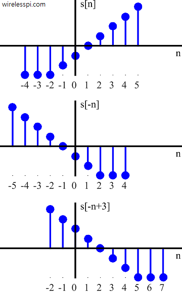
Note that the rules of shifting to the left or right also become reverse due to the flipped time-axis, $-n$, itself. For example, from the perspective of intuitive method above, an axis of $-n$ instead of $n$ suggests that the past becomes the future, and vice versa. Hence, $s[-n+3]$ first flips the signal around time origin, then travels $3$ units to the past to label it the new NOW (time index $0$).
Circular Shift
Circular shift is very similar to time shifting of a signal, except that the available axis for time shifting a signal is from $-\infty$ to $+\infty$ while we only focus on a segment of $N$ samples for a circular shift.
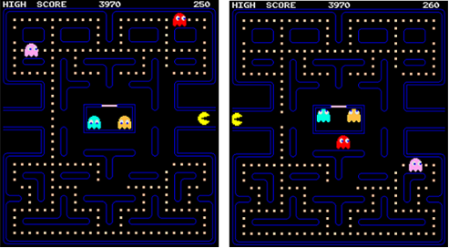
If a signal $s[n]$ is circularly right shifted by $m$, the samples of the signal $s[n]$ that fall off to the right of length-$N$ segment reappear at the start. Similarly, if $s[n]$ is circularly left shifted by $m$, the samples of the signal $s[n]$ that fall off to the left of length-$N$ segment reappear from the end. Just like a video game character which disappears at one end of the screen to emerge from the other. An example for Pacman circularly shifting to the right is shown below.

A simple rule to remember circular shift is "what goes around comes around".
As circular shift is done with respect to a length-$N$ segment, shifts are computed modulo $N$ and denoted as $s[(n-m) \:\text{mod}\: N]$, where $(n-m)\: \text{mod} \:N$ means shifting the signal as we normally would, but bringing them back in the range $0\le n \le N-1$ from the opposite side. For example, the next Figure shows two examples of circular shifts:
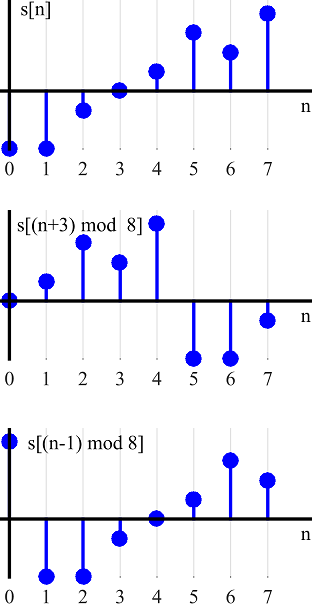
- $s[(n-1) \:\text{mod}\: 8]$ is a right shift of $1$ in every respect, except for sample at time index $7$. Instead of going to index $8$, it returns from the left at index $0$.
- Again, $s[(n+3) \:\text{mod}\: 8]$ is a left shift of $3$ for most samples, except for samples at time indices $0$, $1$ and $2$. Instead of going to negative time, these three samples return from the right at indices $5$, $6$ and $7$, respectively.
As an exercise, try drawing $s[(n+7) \:\text{mod}\: 8]$ and $s[(n-5) \:\text{mod}\: 8]$. You will find that these shifts are actually the same as $s[(n-1) \:\text{mod}\: 8]$ and $s[(n+3) \:\text{mod}\: 8]$, respectively.
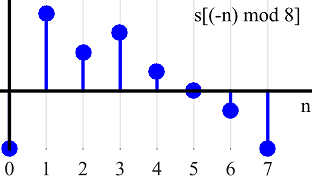
An interesting question at this stage is: what will be the result of a circularly flipped signal $s[(-n) \:\text{mod}\: N]$? The logic of circular shift stays the same. Like regular flipping, the sample at index $0$ remains fixed. The sample at index $7$ should take a position at $-7$ but there is no negative indexing in circular notation and $(-7) \:\text{mod}\: 8 = -7+8 = 1$, which takes it to index $1$. Figure below shows $s[(-n) \:\text{mod}\: N]$ $=$ $s[-n+N]$ for the same signal as above.
The significance of circular shift will become clear when we discuss the Discrete Fourier Transform (DFT) later.
Thanks for such a nicely presented visual explanation.