In this article, we describe the free space propagation in mmWave systems. During the discussion, we dispel a common myth that the received power at any distance decays with increasing carrier frequency. We will see that the received power is in fact independent of the carrier frequency for suitably designed systems such as those at mmWave frequencies. Instead, it is only after including the atmospheric effects such as water vapors, oxygen, rain and penetration loss in materials that the carrier frequency plays a substantial role in establishing the link budget.
Suppose that a Tx transmits $P_{\text{Tx}}$ watts of power uniformly radiating in all spatial directions. Taking the Tx as a point source, the power radiates outwards in every dimension, i.e., in a sphere, which is known as isotropic radiation. Then, the power density at a distance $d$ from the Tx point source is the ratio of the Tx power $P_{\text{Tx}}$ to the surface area of the sphere $4\pi d^2$.
\[
\text{Power density} = \frac{P_{\text{Tx}}}{4\pi d^2}
\]
This is for an ideal isotropic antenna. Now if the gain of the real Tx antenna towards the Rx is given by $G_{\text{Tx}}$, the above expression becomes
\[
\text{Power density} = \frac{P_{\text{Tx}}}{4\pi d^2}\cdot G_{\text{Tx}}
\]
This gain factor accounts for the losses from a real antenna as well as its directionality: it is the ratio of the radiation intensity in a given direction to the radiation intensity that would be obtained for an isotropic antenna emitting equal power in all directions.
Next, assume that the Rx antenna has an effective aperture given by $A_E$ which determines the amount of incident power collected at the Rx side. Therefore, $P_{\text{Rx}}$ can be written as the product between the power density and effective aperture.
\begin{equation}\label{equation-prx-aperture}
P_{\text{Rx}} = \text{Power density}~\times~A_E = \frac{P_{\text{Tx}}}{4\pi d^2}\cdot G_{\text{Tx}} \cdot A_E
\end{equation}
From antenna theory, this effective aperture is given by the expression below.
\begin{equation}\label{equation-antenna}
A_E = G_{\text{Rx}}\cdot \frac{\lambda^2}{4\pi}
\end{equation}
where $\lambda$ is the carrier wavelength and $G_{\text{Rx}}$ is the Rx antenna gain. Therefore, we have
\begin{equation}\label{equation-prx-total}
P_{\text{Rx}} = \frac{P_{\text{Tx}}}{4\pi d^2}\cdot G_{\text{Tx}} \cdot G_{\text{Rx}}\cdot \frac{\lambda^2}{4\pi}
= \frac{P_{\text{Tx}}}{(4\pi d)^2}\cdot G_{\text{Tx}} \cdot G_{\text{Rx}}\cdot \lambda^2
\end{equation}
There are two opposing factors at interplay in the above expressions.
Scenario I
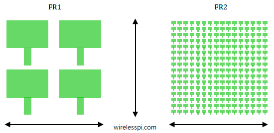
From Eq (\ref{equation-prx-total}), we observe that the Rx power in free space increases with $\lambda^2$, the squared wavelength. Since wavelength has an inverse relation to frequency, or $\lambda=c/F_C$, another way of saying this is that the signal power decreases in proportion to $F_C^2$, the squared carrier frequency. To understand this idea intuitively, consider two antenna arrays, one operating at low or mid band FR1 and the other at high band FR2. For the same number of antenna elements and antenna spacing with respect to the wavelength (e.g., $\lambda/2$), the antenna array at high band will be significantly smaller than the antenna array at low or mid bands. This is drawn in the figure below where two antenna arrays, both of which have a similar gain, are shown. This is similar to a window in your room: the larger the window size, the higher the amount of sunshine captured.

Let us compare this path loss at a distance $d=50$ meters in a representative set of frequencies for equal Tx power, omnidirectional antennas and, most importantly, unit Tx and Rx gains $G_{\text{Tx}}=G_{\text{Rx}}=1$.
\[
\begin{aligned}
F_C = 900 \text{ MHz} \qquad& \longrightarrow \qquad -65 \text{ dB} \\
F_C = 2.4 \text{ GHz} \qquad& \longrightarrow \qquad -74 \text{ dB} \\
F_C = 5.8 \text{ GHz} \qquad& \longrightarrow \qquad -82 \text{ dB} \\
F_C = 60 \text{ GHz} \qquad& \longrightarrow \qquad -102 \text{ dB}
\end{aligned}
\]
In words, operating in mmWave band requires the designer to compensate for around 20-40 dB of Rx power loss in comparison to the lower microwave frequencies. Fortunately, this is possible if we note that this frequency dependence is a pure antenna effect. Otherwise, a high frequency electromagnetic wave itself suffers no extra attenuation while propagating from the Tx to a Rx in the far field region.
Scenario II
The increased attenuation at higher frequencies is largely due to the assumption of constant gains $G_{\text{Tx}}$ and $G_{\text{Rx}}$ above that is a result of reducing the antenna size with the decreasing wavelength at high band. Now if the area of the antenna array is kept constant regardless of the wavelength and the element spacing is again fixed at, say $\lambda/2$, then more number of antenna elements are required to cover the same physical space. This is drawn in the figure below where the array now consists of a significantly larger number of elements. An increase in the array elements thus increases the Tx and Rx gains.

What is the effect of final received power $P_{\text{Rx}}$? From Eq (\ref{equation-antenna}), the gain is inversely proportional to $\lambda^2$.
\[
G_{\text{Rx}} \propto \frac{1}{\lambda^2}
\]
Plugging this in Eq~(\ref{equation-prx-total}), we get
\[
P_{\text{Rx}} \propto \frac{P_{\text{Tx}}}{(4\pi d)^2}\cdot G_{\text{Tx}} \cdot \frac{1}{\lambda^2}\cdot \lambda^2 = \frac{P_{\text{Tx}}}{(4\pi d)^2}\cdot G_{\text{Tx}}
\]
The effect of wavelength or frequency is thus completely eliminated! In fact, if similar antenna arrays are used at both sides of the link, i.e., at the Tx side too thus changing $G_{\text{Tx}}$, then the received power can be increased at high band! The coverage at mmWave frequencies can in fact become better in free space than sub-6 GHz frequencies.
To consider the effect of gain in terms of actual numbers, a system with $1000$ Watts of Tx power along with a gain of $10$ (10 dB) provides the power equal to
\[
1000\times 10 = 10000
\]
This number is the same as $100$ Watts of Tx power along with a gain of $100$ (20 dB).
\[
100\times 100 = 10000
\]
In reality, while a higher gain is achieved through a large number of antennas at mmWave frequencies that adequate provide the coverage, the allowed output power is still limited and the coverage area is usually smaller than sub-6 GHz frequencies.
To summarize, higher attenuation at mmWave frequencies can be compensated for, and even surpassed, through highly directional antennas as it is easier to increase the Tx and Rx antenna gains than the Tx power in mmWave systems. This is the principle on which mmWave communication is based where increased directivity is provided by massive MIMO and beamforming in 5G systems. The interesting point to note is that antenna array in a massive MIMO system requires a reasonably small form factor due to the dependence of antenna spacing on very short wavelengths. As a consequence, it forms a natural partnership with mmWave frequencies for transmissions at Gbps.