We have seen in the effect of phase rotation that the matched filter outputs do not map back perfectly onto the expected constellation, even in the absence of noise and no other distortion. Unless this rotation is small enough, it causes the symbol-spaced optimal samples to cross the decision boundary and fall in the wrong decision zone. And even for small rotations, relatively less amount of noise can cause decision errors in this case, i.e., noise margin is reduced. In fact, for higher-order modulation, the rotation becomes even worse because the signals are closely spaced with each other for the same Tx power. Similarly, sampling the incoming Rx signal anywhere other than the zero-ISI instants causes inter-symbol interference (ISI) among neighbouring symbols. A synchronization unit is vital to ensure the proper functionality of a wireless communication system. We explain the fundamental problem of synchronization through the help of the phase rotation impairment.
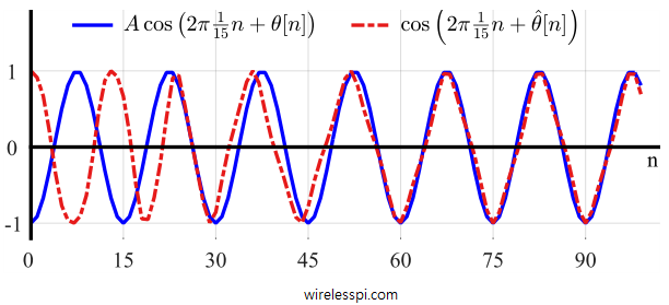
Usually, a PLL expects a continuous wave at its input, the phase of which can easily be locked onto. See a locking example of a PLL input and output below.
Imagine a QPSK signal input directly into a PLL designed to estimate and compensate for the phase and frequency of a sinusoid. Instead of the rectangular IQ expression you see for linear modulations, we can write a passband QAM waveform in polar form as
$$ s(t) = \sum _m \sqrt{a_I^2[m] + a_Q^2[m]} \cdot p(t-mT_M) \cdot \sqrt{2} \cos \left(2\pi F_C t+ \tan^{-1}
\frac{a_Q[m]}{a_I[m]}\right) $$
In this polar form, we have a single sinusoid whose amplitude is fixed for PSK modulation and phase is determined by symbols $a_I[m]$ and $a_Q[m]$.
The modulated signal arriving at the Rx consists of two different phase components:
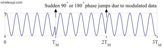
- Unknown phase shifts arising due to modulating data occurring at symbol rate $R_M$. For example, in BPSK modulation, phase changes by $0^\circ$ or $180^\circ$ at the boundary of each symbol interval $T_M$. For QPSK, there are four different phase shift possibilities, i.e., $45^\circ$, $135^\circ$, $-135^\circ$, or $-45^\circ$. A similar argument holds for Quadrature Amplitude Modulated (QAM) signals as well.
- Unknown phase difference between Tx and Rx local oscillator, $\theta_\Delta$.
Depending on its design parameters, the PLL will try to lock onto the incoming phase within a specific time duration. However, that phase is jumping around by $0^\circ$, $\pm 90^\circ$ or $180^\circ$ at every symbol boundary due to modulating data, never allowing our mechanism to converge. This is the fundamental problem every synchronization subsystem needs to address and is illustrated in Figure below.

Now we try to locate the pulse shape in this phase recovery process. First, the carrier does not need to be involved in this process. With the expansion of unique digital processing solutions and shrinking of the analog side in the wireless communication systems, the signal is downconverted by a free running oscillator at a fixed frequency (leading to low phase jitter) and the phase offset can be compensated in the IQ modulated data right there and then.
Most timing synchronization algorithms operate independent of the phase information. Therefore, almost all the DSP based carrier phase synchronization algorithms are timing-aided which means that the symbol boundaries in the Rx sampled waveform are established before the phase recovery block. Knowing the exact symbol boundaries is the same as identifying the optimal sampling instants where the eye opening is maximum and Inter-Symbol Interference (ISI) from the neighbouring symbols is zero. An example of a matched filter IQ output is drawn in Figure below.
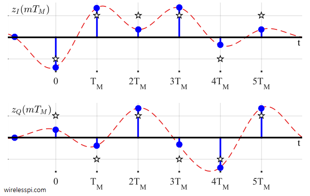
You can see the Raised Cosine pulse shape in the background as a red line.
Many SDR enthusiasts outside of the core wireless area find it strange when they encounter a carrier phase synchronization block of code (e.g., a PLL or a Costas loop in GNU Radio) in which there is no `carrier’ to be compensated for! Instead, they only find a phase de-rotation of the IQ samples going into the symbol detector as shown above.
When you implement an actual phase synchronizer, a small frequency offset can also be present in this signal. For example, if the carrier was off by 1 Hz, this phase rotator would be spinning at a 1 Hz rate as we saw before in the article on the effect of frequency offset. This implies that the complex baseband (I and Q) are different than what was received at the actual carrier frequency. If the carrier is still there, it is due to the carrier frequency offset, and not the actual carrier frequency.
From here, a phase error detector removes the modulation such that the input to the loop filter is a track-able signal. All in all, the task of a phase synchronization unit in a Rx is to estimate this phase offset and de-rotate (since the rotation of a complex number is defined with respect to anticlockwise fashion, de-rotation implies rotating the input in a clockwise direction) the matched filter outputs by this estimate either in a feedforward or a feedback manner. In such a way, the carrier at the Rx can be said to become synchronized with the carrier used at the Tx.
We are faced with two options in this situation. Either transmit the synchronization signal in parallel to the data signal that costs increased power and/or bandwidth, or some procedure needs to be invoked to remove the modulation induced phase shifts in the data signal as a result of which
[for a phase offset] the output should become a constant complex number whose phase is our unknown parameter, and
[for a frequency offset] the output should become a simple complex sinusoid whose frequency is our unknown parameter.
Then, either a feedforward (one-shot) estimator or a feedback mechanism (a PLL) can detect this unknown phase. We can either utilize this observation directly to come up with some intuitive phase estimators, or employ our master algorithm — the correlation — to this problem and see where it leads. Interestingly, it turns out that the derivation of phase estimators through the maximum correlation process actually leads to the same intuitively satisfying results. Maximum correlation is a result of a procedure termed as maximum likelihood estimation. Almost all ad hoc synchronization algorithms can be derived through different approximations of the maximum likelihood estimation. For Gaussian noise under some constraints, maximum likelihood and maximum correlation are one and the same thing.
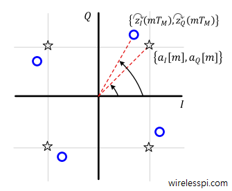
Suppose that the training symbols $a_I[m]$ and $a_Q[m]$ are known (a data-aided system), then their angle can be subtracted from the angle of the matched filter output at each symbol time as
\begin{equation}
\hat\theta_\Delta[m] = \measuredangle~ \frac{z_Q(mT_M)}{z_I(mT_M)} – \measuredangle ~\frac{a_Q[m]}{a_I[m]}
\end{equation}
The intuition this approach is simple: the phase difference between received and expected symbols is the remaining phase offset.