Alfred North Whitehead said,
In today’s world, it is easy to take no notice of the level of process automation integrated into our lives. To have an idea of how things were in the early days, signal processing technology to sort out the radar picture on a map was not available and only a dot or a line could be generated on the screen representing a detected target. A radar operator had to stare at a screen for their whole shift to raise a warning when a blip appeared on the screen, see an example below.
Image credit: Plate V, J.G Crowther and R Whiddington, Science at War, London: HMSO, 1947; Crown Copyright expired

This could have easily been the most boring job ever in the world. Except that these pioneers did not know that billions of humans of the next century would happily walk into their footsteps by spending most of their professional and personal lives staring into the screens.
Background
Today signal processing offers us automation of tasks much more complicated than detecting a simple blip. For example, recall that an incoming wireless signal at a receiver (Rx) varies significantly over time in both phase and amplitude. These variations are on top of the linear modulations forced by the transmitter (Tx) and hence must be compensated for before the final decision about the underlying digital symbol. Just like a Phase-Locked Loop (PLL) automatically tracks the carrier phase of this wireless signal in a feedback loop, an Automatic Gain Control (AGC) performs a similar task for the amplitude. It tracks and compensates for the amplitude variations arising, for example, due to multipath fading and movement, and adjusts the Rx gain according to an average level prescribed by the designer.
But why do we need to control the signal amplitude around a certain level? This is due to its crucial role in various detection tasks down the chain, some of which are as follows.
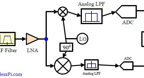
- In the discussion on analog to digital conversion, we saw that there is a performance penalty if the peak amplitude of the waveform is below the full-scale ADC amplitude. Boosting this peak amplitude towards the ADC full-scale voltage utilizes the full dynamic range available. On the other hand, if the incoming analog signal has a peak amplitude larger than the peak ADC voltage, clipping along with non-linear distortion effects arise. For this purpose, an AGC is implemented in analog domain before the ADC, the design of which is beyond the scope of this article.
- As far as a digital AGC is concerned, recall that for linear modulations like Phase Shift Keying (PSK) and Quadrature Amplitude Modulation (QAM), the decision region and its boundaries at the receiver are drawn according to an average received signal level. As soon as this average level starts varying, we have a time-varying Rx decision region on our hands which is bound to be different than the Tx constellation. This leads to an increased symbol error rate. Such a problem can be fixed by maintaining an average signal level at the start of the DSP chain that in turn results in a stable Rx decision region with time-invariant boundaries for symbol detection.
- In many receivers, a carrier Phase Locked Loop (PLL), a timing PLL and a Frequency Locked Loop (FLL) are used for synchronization purpose. A loop filter is an integral component of these PLLs that determines the loop bandwidth and subsequently its performance. The design of this filter requires computation of the phase error detector gain that in turn depends on the average symbol level. Consequently, a time-varying signal amplitude produces a loop with time-varying loop bandwidth and hence a behavior not intended by the designer.
In the light of the above, a digital AGC is designed to dynamically adjust the input signal amplitude, instead of changing the decision regions of the constellation as well as the loop constants. Remember that an AGC does not drown out the digital modulation on each symbol; instead it maintains an average signal level during the communication. Let us turn our attention now towards its operation.
AGC Operation
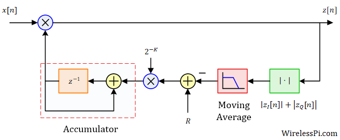
In principle, an AGC is a feedback control system that drives the amplitude error to zero in an iterative fashion. This establishes, on average, a constant signal amplitude at the start of the DSP chain. To see how this is accomplished, consider the block diagram below.

The input signal is $x[n]$ that is multiplied with the AGC output $a[n]$, thus producing the output $z[n]$. In the feedback loop, the magnitude of the complex signal $z[n]$ is found as
\[
|z[n]| = \sqrt{z_I^2[n] + z_Q^2[n]} = |a[n-1]\cdot x[n]|
\]
The reference level $R$ is where we want the output $z[n]$ to settle after AGC convergence. To accomplish this task, an error signal is produced as
\begin{equation}\label{equation-agc-error}
e[n] = R ~-~ \big|a[n-1]\cdot x[n]\big|
\end{equation}
Finally, the amplitude update expression can be written as
a[n] = a[n-1] +\mu \cdot e[n]
\]
The above familiar expression is very similar to the Least Mean Square (LMS) update equation which is a special case of an adaptive algorithm. Clearly, when the input signal level is high, a negative voltage is fed back, see the error expression above, thus reducing the gain that brings the signal level down after multiplication. A similar operation is performed to increase the gain when the input signal level is low.
Solving the AGC Equation
Let us expand the above AGC equation by plugging in the value of error signal $e[n]$ from Eq (\ref{equation-agc-error}). To model a sudden change in amplitude, we assume that the input signal is a constant jump from zero to a positive value $B$, i.e., $x[n] = B u[n]$ where $u[n]$ is the unit step signal.
\[
a[n] = a[n-1] +\mu \cdot \Big\{R ~-~ a[n-1]\cdot B\Big\}, \qquad n \ge 0
\]
This can be arranged as
\[
a[n] = \big(1-\mu B \big)a[n-1] + \mu R
\]
The above expression is a linear difference equation that can be solved using the linearity principle as
a[n] = \left\{a[0] ~-~ \frac{R}{B}\right\}\left(1-\mu B\right)^n + \frac{R}{B}
\]
where the initial value $a[0]$ can be taken as 1. As $n$ goes to infinity, the first term vanishes and the steady state value of $a[n]$ can be seen as $R/B$. When this value is multiplied with the input signal, which is a constant $B$, we get
\[
z[n] = \frac{R}{B}\cdot B = R
\]
In words, the output is a signal with a constant amplitude $R$, the set reference! Generalizing this result where the input signal is not a simple unit step, it is clear that the output signal still has an amplitude given by $R$.
Convergence Time
Notice from the AGC expression above that the factor that goes to zero with time is given by $\left(1-\mu B\right)^n$, which depends on the input signal amplitude! Convergence is one of the major issues in all feedback systems. In this scenario, a signal can only move forward in the processing chain after the AGC has converged. Since this is accomplished during the preamble processing that contains known symbols, a slow AGC necessitates a longer preamble that is inefficient for bandwidth utilization. Moreover, the loop can lose track during rapid signal fading that can restart the acquisition process. Consequently, the AGC loop settling time should be signal independent for optimal operation.
Skipping the mathematical derivation of such a phenomenon for simplicity, let us observe the performance when the input signal $x[n]$ is given by
\[
x[n] = B_n e^{j2 \pi f_0n}
\]
where $f_0$ is the discrete frequency equal to $F_s/20$ while $B_n$ is a time-varying amplitude.
\[
B_n =
\begin{cases}
1 & \qquad 0 \le n \le 250 \\
0.1 & \qquad 251 \le n \le 500 \\
1.5 & \qquad 501 \le n \le 750\\
0.4 & \qquad 751 \le n \le 1000
\end{cases}
\]
The input and output signals, $x[n]$ and $z[n]$, respectively, are shown in the figure below for the reference level $R=1$ and the step size $\mu=0.1$. The bottom subfigure plots them overlapped on each other for a clear demonstration of convergence times.

Some comments regarding the above figure are in order.
- Notice that the output tracks the input nicely during the 1st quarter of the above figure where $B_n=1$.
- However, during the 2nd quarter where $B_n=0.1$, it takes a long time for the AGC to converge towards reference level $R=1$. In fact, it has not converged even at the end of the said interval. This can be a severe problem for a digital wireless system where the AGC cannot catch up with rapidly changing signal fading, resulting in disastrous performance of tracking loops and errors in symbol decisions.
- During the 3rd quarter where $B_n=1.5$, the AGC converges quickly converges to the desired steady-state value.
- For the 4th quarter where $B_n=0.4$, the output signal approaches the input utilizing a time somewhere between the 2nd and 3rd quarters.
All this demonstrates that the convergence time of the AGC depends on the signal level. During the high-amplitude intervals, the output signal tracks the input without a significant delay. On the other hand, during low-amplitude intervals, all the DSP down the chain has to wait before the convergence is achieved.
This convergence is characterized by a time constant $n_0$ which is defined as the time during which the AGC output $a[n]$ approaches $(1-e^{-1})$ of its steady-state value ($R/B$ in the above example). The time constant is large during low amplitude intervals and small during high intervals. This becomes more clear when we draw the AGC gain $a[n]$ and the error signal $e[n]$ in the figure below corresponding to the example discussed above. Observe the slow gain $a[n]$ convergence during the 2nd quarter where the signal amplitude was low and fast convergence in the 3rd quarter where the amplitude was high.

An introduction to slow and fast attack AGCs is given below.
- Slow Attack AGC uses a small value of $\mu$, implying that the gain changes gradually over time. This helps maintain stability and prevents rapid fluctuations.
- Fast Attack AGC uses a larger value of $\mu$, allowing the gain to adjust quickly to sudden changes in signal amplitude. This is useful for handling abrupt signal variations.
In practical implementations, AGC systems may also incorporate adaptive attack rates, where the attack speed changes depending on the signal conditions. During signal acquisition, a fast attack AGC is typically used to expedite the process, although it compromises noise performance. Once the signal is acquired, the AGC control loop operates at a slower rate, improving noise performance while remaining responsive enough to track signal dynamics in a robust manner.
Next, we mention some techniques better suited to practical implementation of the AGC.
Implementation Details
There are a few techniques that can result into an efficient implementation, some of which are described below.
- In some implementations, such as the one shown in the figure below, the step size $\mu$ can be treated as a dynamic parameter that can be configured on the fly. Choosing it as a power of two, such as $2^{-K}$ shown in this figure, saves memory and computations.

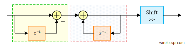
- Also, a moving average filter can be inserted after the magnitude computation to smooth out the transitions and prevent the AGC to attempt level correction far too often, as drawn in the figure above. Here, instead of a conventional moving average, a combination of a comb and an integrator can be used in a similar manner as Cascaded Integrator Comb (CIC) filters. A block diagram of this comb and the integrator is illustrated in the figure below. Choosing the filter length $L$ as a power of two implies that the filter scaling at the end can be achieved through a simple right shift as an efficient alternative to a division operation.
- From a computational viewpoint, the most critical part of the AGC loop is the magnitude operation. For a complex signal, this is implemented with the help of two multipliers, one addition and one square-root operation, as illustrated in the figure below. Multiplication and square-root (even if implemented through a Coordinate Rotation Digital Computer (CoRDiC) for efficiency) are not desirable operations in resource-constrained wireless devices. Therefore, an efficient implementation from [1] is also plotted in the same figure that approximates the magnitude as
\[
\sqrt{z_I^2[n]+z_Q^2[n]} \approx |z_I[n]| + |z_Q[n]|
\]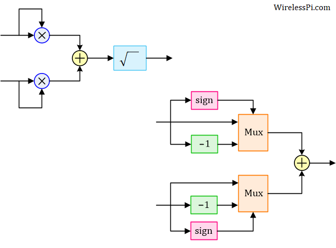
This absolute value is computed as follows. A mux selects one of two values based on the sign of the input. If the value is positive, the mux simply sends it forward. Otherwise, its sign is inverted.


A part of a sample script is shown in the figure below.

Let us now discuss a log AGC that solves the slow convergence problem for low amplitude intervals.
Log AGC
We saw above that the convergence time of the AGC depends on the signal amplitude. For high signal levels, it quickly reaches the steady-state value while the journey is much slower during low signal levels. This delay is detrimental for the subsequent signal processing blocks. To see how this issue can be handled, consider the block diagram of a log AGC shown in the figure below.

Observe three changes as compared to a linear AGC covered above: It is the log of the magnitude that is of interest, the reference level is changed to $\log (R)$ and there is an antilog operation before the AGC delivers its output for gain control.
To understand its operation, start with the input signal $x[n]$ that is multiplied with the AGC output $a[n-1]$, thus producing the output $z[n]$. The reference level is $\log(R)$ but the output $z[n]$ settles to $R$ after AGC convergence. Clearly, the error signal is produced as
\begin{equation}\label{equation-agc-error-log}
e[n] = \log(R) ~-~ \log\left(\big|a[n-1]\cdot x[n]\big|\right)
\end{equation}
because the logarithm is taken after the output magnitude operation. Now the amplitude update expression can be written as
\log(a[n]) = \log(a[n-1]) +\mu \cdot e[n]
\]
Why? Because the accumulator output is generated before the antilog operation, i.e., $\exp(x)=a$ implies that $x=\log(a)$. Again, let us plug in the value of error signal $e[n]$ from above and assume that the input signal is a constant jump $x[n] = B u[n]$ where $B$ is positive.
\[
\log(a[n]) = \log(a[n-1]) +\mu \cdot \Big\{\log(R) ~-~ \log\left|a[n-1]\cdot B\right|\Big\}, \qquad n \ge 0
\]
Using $\log(a[n-1]\cdot B)=\log(a[n-1])+\log(B)$, this can be rearranged as
\[
\log(a[n]) = \left(1-\mu \right)\log(a[n-1]) ~+~ \mu \log\frac{R}{B}
\]
Again, the above expression is a linear difference equation that can be solved using the linearity principle as
\[
\log(a[n]) = \left\{\log(a[0]) ~-~ \log \frac{R}{B}\right\}\left(1-\mu \right)^n + \log\frac{R}{B}
\]
For a zero initial condition, $a[0]=1$ and the above equation reduces to
\log(a[n]) = \log \frac{R}{B}\big\{1-\left(1-\mu \right)^n\big\}
\]
Clearly, the factor that goes to zero with time is given by $\left(1-\mu\right)^n$, which is independent of the input signal amplitude $B$! This is in opposition to what we observed in the case of a linear AGC before where the time-dependent term was $\left(1-\mu B\right)^n$. This behavior is evident from the input and output signals in the figure below. The output is seen to be reaching the steady-state regardless of different signal levels in all four quarters.

The gain and error curves tell the same story where a fast convergence is observed in 2nd quarter despite the signal level being only equal to $0.1$.

Finally, we turn towards a feedforward implementation of the AGC.
Feedforward AGC
While feedback AGCs are mostly used, designing a feedfoward AGC is also possible. A block diagram of such a module is drawn in the figure below which is simpler than its feedback counterpart. The magnitude operation is again approximated through absolute values. After the moving average filter, a reference level $R$ is divided by the input signal magnitude so that when it is multiplied with the input signal in the next step, the output signal is automatically set to amplitude $R$. The division can be efficiently implemented here through a CoRDiC.

The input and output signals are drawn in the figures below where the output can be seen as quickly following the input variations.
The gain plot below also tells us that convergence time is irrelevant for the feedforward AGC. As long as the signal does not vary too fast compared to the sample rate, a satisfactory performance


In a properly designed system, both feedback and feedforward AGCs deliver an equivalent performance.
Conclusion
An Automatic Gain Control (AGC) is the amplitude analog of a Phase Locked Loop (PLL). In this article, we discussed a few different kinds of AGC. A linear AGC suffers from the dependence on the input signal amplitude which results in variable convergence times, thus limiting its utility in practical applications. On other hand, a log AGC tracks the input signal within a prescribed time, regardless of the signal level. Therefore, a log AGC is commonly employed in wireless communication systems. A feedforward AGC configuration is also possible.
References
[1] K. Sobaihi, A. Hammoudeh, D. Scammell, Automatic Gain Control on FPGA for Software-Defined Radios, Wireless Telecommunications Symposium (WTS), April 2012.
Hi,
The opening remarks on the need of AGC mentions Analog and Digital implementation of AGC. Does a Rx has AGC in both analog (before ADC) and digital domains?
In general, yes, that’s correct.
I would assume analog AGC should keep the signal within dynamic range of the ADC and this digital AGC should keep the signal constant for the PLL/FLLs?
Yes that’s largely correct.
Very good article! You explore nice alternatives.
Also you can approximate the calculation for the amplitude of the complex $z$, as follows:
\[
\text{abs}(z) = \frac{7}{8}\text{max(abs(real}(z)), \text{abs(imag}(z))) + \frac{1}{2}\text{min(abs(real}(z)), \text{abs(imag}(z)))
\]
[1] “An improved Digital Algorithm for Fast Amplitude Approximations of Quadrature Pairs”
Good point. Thanks
The Log AGC algorithm has to handle logarithmic and exponential operations, which are quite complex. Is there any high-performance numerical operation method suitable for engineering implementation?
Such operations can be implemented through lookup tables if memory is available or CoRDiC algorithm if computations can be afforded.
Thank u for good suggestions
Is the code implementation? and does it work for audio signal? and why is the z[n] is complex signal, does it work for real-valued signal?
Yes it works for audio signals and real signals.
Great explanation of AGC and how it functions in wireless systems! I appreciate the clarity in your examples. It really helped me understand the importance of maintaining signal quality. Looking forward to more posts like this!
This is a really informative post! I had a basic understanding of AGC, but your detailed explanations and examples clarified a lot for me. It’s fascinating to see how AGC optimizes signal quality in different environments. Thanks for sharing!
Great explanation of AGC! It’s fascinating how it helps maintain consistent audio levels. I didn’t realize it also plays such a crucial role in wireless communication. Thanks for breaking it down so clearly!
Hi, Qasim!
It’s very cool article! And very cool, that you can download it! Thank you!
What about the fast attack mode and slow attack mode in ADC AGC gain controller? Any thoughts on Hysteresis? To complement your good theory, ADI9361/9371 in MATLAB/Simulink can also be referred to study AGC implementation in high speed ADC for wireless applications
Thanks Rahul for the feedback. Yes, these are definitely interesting and relevant topics which you pointed out. However, this tutorial is written from a fundamentals perspective.
Great explanation of AGC! I never realized how crucial it is for maintaining audio quality in wireless communication. The diagrams really helped clarify the concepts too. Thanks for breaking it down!
Great explanation of AGC! I appreciate how you broke down the technical aspects into understandable terms. It’s fascinating to see how this technology optimizes audio levels in real-time. Looking forward to more posts like this!
Great explanation of AGC! I never realized how crucial it is for maintaining consistent audio levels in wireless systems. The examples really helped clarify its practical applications. Thanks for shedding light on this!
Great explanation of AGC! I appreciate how you broke down the technical aspects and made it easy to understand. It’s fascinating how this technology enhances wireless communication. Looking forward to more insights like this!