A Phase Locked Loop (PLL) is a device used to synchronize a periodic waveform with a reference periodic waveform. It is an automatic control system in which the phase of the output signal is locked to the phase of the input reference signal.
- In the context of carrier phase synchronization, we talk about tracking the phase of an input reference sinusoid.
- For carrier frequency synchronization, a Frequency Locked Loop (FLL) is implemented.
- For the purpose of timing synchronization, the target is to adjust the timing phase of a receiver clock to that of the transmitter clock such that one sample/symbol required for symbol detection is taken at the maximum eye opening.
PLL Structure
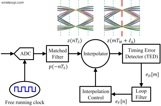
A PLL employed for digital timing recovery consists of the following components, a block diagram of which is drawn in the figure below. The notations for the main parameters are the following.
- Sample time (inverse of sample rate): $T_S$
- Matched filter output: $z(nT_S)$ where $n$ is an integer
- Symbol time (inverse of symbol rate): $T_M$
- Timing error: $\epsilon _\Delta$
- Timing error estimate at Rx: $\hat \epsilon _\Delta$
- Matched filter output at 1 sample/symbol: $z(mT_M+\hat \epsilon_\Delta)$ where $m$ is an integer
- Square-root Raised Cosine pulse shape: $p(nT_S)$

At the receiver, the arriving signal $r(t)$ is sampled by a free running clock at a constant rate $1/T_S$ that is asynchronous to the symbol rate $1/T_M$ as shown in the figure above. These samples $r(nT_S)$ are matched filtered to produce $z(nT_S)$ at $L$ samples/symbol, none of which lies at the symbol boundary, i.e., an integer multiple of $T_M$. Here, the job of the timing synchronization loop is twofold.
- Figure out an estimate of the timing offset $\hat \epsilon _\Delta$ (or an error signal $e_D[m]$ proportional to it).
- Then, rather than shifting a physical clock (such as a voltage controlled clock that exhibits excessive phase noise and delay), construct the `missing samples’ at optimal locations $z(mT_M +\hat \epsilon _\Delta)$ by an algorithm operating on asynchronous samples $z(nT_S)$. This process is known as interpolation. The economic advantage of digital processing and a free running clock made this option the most viable in software defined radios.
Timing Error Detector (TED)
A timing error detector solves the fundamental problem of synchronization. While the input is a sinusoid in a carrier PLL, as we saw during phase synchronization, the corresponding input here is the matched filter output $z(nT_S)$. A Timing Error Detector (TED) generates an error signal $e_D[m]$ during each symbol interval using the matched filter outputs $z(nT_S)$ proportional to the timing phase difference $\epsilon_\Delta$ between the actual and desired sampling instants. The PLL functions properly as long as the mean error has the same sign as the actual error. Most of the timing error detectors operate at $1$ or $2$ samples/symbol. Some of the examples are early-late, zero-crossing and Mueller and Muller timing error detectors.
Loop filter
A loop filter sets the dynamic performance limits of a PLL as well. Moreover, it helps filter out noise and irrelevant frequency components generated in the timing error detector. Its output signal is denoted as $e_F[n]$. The sample index $n$ is the same as the symbol index $m$ for a TED using $L=1$ sample/symbol.
Interpolation control and interpolator
Taking $e_F[n]$ as an input, an interpolator control determines two values, the integer sample closest to the maximum eye opening (called the basepoint index) and the interval between this basepoint index and the optimal sampling instant (known as the fractional interval). Then, these two values are provided to the interpolator. The interpolator control also incorporates a symbol timing frequency difference that slowly traces the difference between the Tx and Rx clock ticks. An interpolator computes the `missing samples’ $z(mT_M+\epsilon_\Delta)$ by using the neighbouring samples $z(nT_S)$.
We now move towards studying the role of timing error detectors in accomplishing this task. The specific technique we cover here is known as the maximum likelihood timing error detector.
Working of a Timing Error Detector (TED)
Just like a phase error detector, a Timing Error Detector (TED) sits at the heart of a feedback loop for timing correction. Before we start, remember that an eye diagram due to its symbol-periodic overlaps is an excellent summary of signal behaviour in time domain, very similar to a spectrum in frequency domain (they both utilize all the available information).
Let us define for a pulse shaped and matched filtered Pulse Amplitude Modulated (PAM) sequence at instants $mT_M$ (where $m$ is an integer and $T_M$ is symbol time):
\begin{align*}
z(mT_M+\hat \epsilon_\Delta) &\rightarrow \text{Matched filtered output at}~mT_M+\hat \epsilon _\Delta \\
\overset{\centerdot}{z}(mT_M+\hat \epsilon _\Delta) &\rightarrow \text{Derivative of the matched filter output (i.e., its slope) at}~mT_M+\hat \epsilon_\Delta
\end{align*}
The derivative at a point is defined as the slope of the line tangent to the curve at that point. To understand the intuition behind this mechanism, the figure below illustrates from an eye diagram perspective how a valid timing error signal is generated.

In reference to this figure, we discuss the following four scenarios.
T1: $\hat \epsilon _\Delta < \epsilon_\Delta$ and $z(mT_M+\epsilon_\Delta)>0$
When the current sampling instant $\hat \epsilon _\Delta$ is earlier than the actual symbol delay $\epsilon_\Delta$, the value $z(mT_M+\epsilon_\Delta)$ in the top left of the figure is naturally lesser than the peak $+A$. Hence, the derivative of the curve is positive at that instant. A positive slope indicates that the estimate $\hat \epsilon _\Delta$ needs to be increased at next update, i.e.,
\begin{equation*}
\hat \epsilon _\Delta(m+1) > \hat \epsilon _\Delta(m)
\end{equation*}
where the sign ‘>’ above means ‘should be greater than’. A timing error detector can thus be formed as
\begin{equation*}
e_D[m] = z(mT_M+\hat \epsilon _\Delta) \cdot \overset{\centerdot}{z}(mT_M+\hat \epsilon _\Delta)
\end{equation*}
So the product of $z(mT_M+\epsilon_\Delta)$ and the derivative $\overset{\centerdot}{z}(mT_M+\hat \epsilon \Delta)$ yields the positive direction in which our symbol timing offset estimate $\hat \epsilon _\Delta$ needs to move. Couldn’t we just use the derivative or slope alone? This will be explained in cases 3 and 4 below.
T2: $\hat \epsilon _\Delta < \epsilon_\Delta$ and $z(mT_M+\epsilon_\Delta)<0$
Consider this case in the above figure. Again, the current value of $\hat \epsilon _\Delta$ is earlier than the actual value but now the derivative at the sampling instant is negative. This is because the symbol value is $-A$ in this case. Consequently, a product of $z(mT_M+\epsilon_\Delta)$ with the derivative yields the positive direction to move $\hat \epsilon _\Delta$.
T3: $\hat \epsilon _\Delta > \epsilon_\Delta$ and $z(mT_M+\epsilon_\Delta)>0$
Looking at this scenario in the above figure, $\hat \epsilon _\Delta > \epsilon_\Delta$ and it needs to be reduced in the next iteration.
\begin{equation*}
\hat \epsilon _\Delta[m+1] < \hat \epsilon _\Delta[m]
\end{equation*}
Here, the symbol value is $+A$ while the derivative is negative. Thus, their product again generates a negative error signal.
T4: $\hat \epsilon _\Delta > \epsilon_\Delta$ and $z(mT_M+\epsilon_\Delta)<0$
From this case in the above figure, we see that the product of $z(mT_M+\epsilon_\Delta)$ and the positive slope produces a negative error term that correctly pulls the sampling instant back.
We conclude that the goal of a timing error detector is to push the sampling instant closer to the center where the eye is maximally open. And hence the above error detector $e_D[m]$, repeated below for convenience, is a valid error signal.
e_D[m] = z(mT_M+\hat \epsilon _\Delta) \cdot \overset{\centerdot}{z}(mT_M+\hat \epsilon _\Delta)
\end{equation}
This is known as a derivative or maximum likelihood Timing Error Detector (TED). In a data-aided version of the derivative TED, the matched filter output $z(mT_M+\epsilon_\Delta)$ is replaced by the actual symbol value $a[m]$.
\begin{equation}\label{eqTimingSyncMLTEDDA}
e_D[m] = a[m]\cdot \overset{\centerdot}{z}(mT_M+\hat \epsilon _\Delta)
\end{equation}
Finally, during a steady state operation, the decisions from the detector can be deployed. Thus, the decision-directed derivative TED is constructed as
\begin{equation}\label{eqTimingSyncMLTEDDD}
e_D[m] = \hat a[m] \cdot \overset{\centerdot}{z}(mT_M+\hat \epsilon _\Delta)
\end{equation}
For example, the symbol decision $\hat a[m]$ for a binary PAM case is
\begin{equation*}
\hat a[m] = A \times \text{sign} \Big\{ z(mT_M+\epsilon_\Delta)\Big\}
\end{equation*}
Role of Data Transitions
Recall from the article on eye diagram that a single transition in an eye diagram gives information about 3 symbols:
- Now: at which the trace passes the current symbol (e.g., $+A$ or $-A$),
- Past: indicated by whether the trace is coming from an upward or a downward path, and
- Future: indicated by whether the trace is heading upward or downward.
With this information in mind, observe from the figure drawn above earlier the following cases where the triplet indicates Past, NOW and Future.
- $\{+-+\}$, or $\{-+-\}$: When data transitions occur both before and after the current symbol, the slope of the pulses in the eye diagram is a reasonably large value at non-optimal instants. This instructs the proper direction to update the estimate $\hat \epsilon _\Delta$ when multiplied with the data symbol.
- $\{+++\}$, or $\{—\}$: For no data transition, there is an approximately horizontal portion of the eye diagram at the top (case $+$) and at the bottom (case $-$). For this scenario, the actual value of the slope will be very small, no matter how far away the current sampling instant is from the optimal location. Consequently, there is no timing information that can be obtained.
- $\{+–\}$, $\{-++\}$, $\{++-\}$, or $\{–+\}$: When there is a data transition followed by no data transition, or no data transition followed by a data transition, the slope of the trajectories does not pass through zero at optimal instants and introduce a little bias in the estimate. However, for a large number of sufficiently random symbols, its effect averages out to zero.
The above discussion suggests that a sufficient density of data transitions is required for timing synchronization to operate.
Implementation
To implement this phase locked loop, the above timing error detector in Eq \eqref{eqTimingSyncMLTED} needs not to compute the derivative of the Rx signal samples in real time. We have two choices here.
- Pass the matched filtered output $z(nT_S)$ through a filter $h(nT_S)$ that computes the derivative of its input in time domain. Here, the matched filter and the derivative filter appear in series.
- Create an alternative filter based on the pre-computed derivative of the matched filter with respect to time. To see why it works, consider a discrete-time differentiator such as the central difference $0.5\{+1,0,-1\}$ that computes the derivative of a signal in time domain.
\begin{align*}
\overset{\centerdot}{z}(nT_S) &= z(nT_S) * h(nT_S) \\
&= \Big\{r(nT_S) * p(-nT_S)\Big\} * h(nT_S)\\
&= r(nT_S) * \underbrace{\Big\{p(-nT_S)*h(nT_S)\Big\}}_{h_{TMF}(nT_S)}
&= r(nT_S) * \left\{-\overset{\centerdot}{p}(-nT_S)\right\}
\end{align*}Here, the left hand side is the derivative of the matched filter output while the right hand side is the convolution of the Rx signal with a filter $h_{TMF}(nT_S)$. Therefore, $h_{TMF}(nT_S)$ is known as a Timing Matched Filter (TMF).
\begin{equation}\label{eqTimingSyncTMF}
h_{TMF}(nT_S) = -\overset{\centerdot}{p}(-nT_S)
\end{equation}With this approach, the matched filter and the derivative matched filter appear in parallel because they both operate on the same input $r(nT_S)$.
As an example, let us construct a timing matched filter for a square-root Nyquist pulse, say a Square-Root Raised Cosine (SRRC), in discrete-time. When $p(-nT_S)$ is convolved with a derivative computing filter, the coefficients of a timing matched filter are generated which are plotted in the figure below. The downsampled output of this filter is $\smash{\overset{\centerdot}{z}(mT_M+\hat \epsilon _\Delta)}$ that is used in the derivative TED of Eq \eqref{eqTimingSyncMLTEDDA}.

Although both approaches above require two filters, the difference is that the serial approach incurs an additional delay because the input for computing the derivative of the matched filter output is not available until the matched filter actually generates this output. A TLL or a PLL is an iterative solution in which any additional delay within the loop impacts its performance and hence the parallel approach of two filters operating on the same input samples at the same time proves more useful.
Remember that an accurate representation of the derivative of a signal needs a sufficiently oversampled input. This makes such a TED a synchronization system where the input sample rate of the two filters is $L$ samples/symbol and the output error signal is generated once per symbol.
Receiver Structure
Finally, we look into the structure of a phase locked loop that incorporates such a timing error detector. A block diagram for implementation of a Rx with a decision-directed setting is shown in the figure below.

The Rx signal $r(t)$ is sampled at a rate of $F_S=L/T_M$ to generate $r(nT_S)$ at approximately $L$ samples/symbol. The matched filter and timing matched filter process $r(nT_S)$ in parallel at the same rate with their respective outputs being $z(nT_S)$ and $\smash{\overset{\centerdot}{z}(nT_S)}$. These two signals form the inputs to their respective interpolators operating in parallel that produce one sample per symbol as commanded by interpolation control block. These two interpolator outputs are $z(mT_M+\epsilon_\Delta)$ and $\smash{\overset{\centerdot}{z}(mT_M+\hat \epsilon _\Delta)}$ where the former is employed to make the decision $\hat a[m]$.
Subsequently, $\hat a[m]$ and $\smash{\overset{\centerdot}{z}(mT_M+\hat \epsilon _\Delta)}$ combine into a timing error detector according to Eq \eqref{eqTimingSyncMLTEDDD} and generate an error signal $e_D[m]$ once per symbol. In case of a non-data-aided operation, the sign block is removed and the matched filter output $z(mT_M+\epsilon_\Delta)$ is directly used instead of $\hat a[m]$ in forming the TED output. This signal $e_D[m]$ is then upsampled by $L$ to create $e_D(nT_S)$ which matches the sample rate $F_S$ of the loop filter and the interpolation control.
Example
Now we examine the implementation of a derivative TED for the following specifications.
\begin{align*}
\text{Modulation} \quad \rightarrow& \quad 2-\text{PAM}, \\ L \quad =& \quad 8 ~\text{samples/symbol}, \\ \alpha \quad =& \quad 0.4, \\
B_n T_M \quad =& \quad 1/200, \\ \zeta \quad =& \quad 1/\sqrt{2}, \\ \epsilon_\Delta \quad =& \quad 0.25 T_M
\end{align*}
With these specifications for a timing locked loop, the Proportional plus Integrator (PI) loop filter coefficients are computed in Eq (4) of the article on PLL implementation in SDRs. For this purpose, the NCO gain $K_0$ and TED gain $K_D$ are also required. We fix $K_0$ as unity while a simple routine is used to compute the derivative of the mean curve at $\epsilon_\Delta=0$ for $K_D$. The output error signal $e_D[m]$ for a derivative TED is shown in the figure below and the estimate of the timing offset $\epsilon_\Delta=0.25T_M$ is seen converging to its true value. This estimate is known as a fractional interval $\mu[m]$. The timing locked loop is seen to converge in approximately $300$ symbols as a result of these design parameters. Observe the abundance of self noise produced by a derivative TED, some of which is inherently present in this TED while the rest is contributed due to the non-data-aided version implemented here.

Concluding Remarks
Finally, a few concluding remarks are in order.
- In most applications, reducing the complexity of the timing locked loop is quite desirable. Instead of having a vastly oversampled Rx signal, a simpler form of a timing error detector is therefore attractive for system design operating at no more than $1$ or $2$ samples/symbol. Due to this reason, there are approximations that have been derived from the above technique such as an early-late timing error detector.
- The timing PLL is not the only route to acquire synchronization. Feedforward schemes that estimate the timing error in one go are also possible, e.g., digital filter and square timing synchronization and maximum likelihood estimation.
- In parallel to a timing locked loop, a certain algorithm known as a lock detector is run which generates a binary output depending on whether the PLL has acquired timing lock or not.
Hello Qasim,
I have a question on Eq.(4), why there is a minus sign before the derivative of p(-nT_s)?
This is because the filter is a flipped version of the pulse shape which implies being a function of -nT_S. Taking the derivative of a function f(-x) implies df/dx times d(-x)/dx where the second term becomes -1.
In the case that we have a symmetric filter such that $p(nT_S) = p(-nT_S)$ as seems to be the case in your drawing, then we would obtain $h_{TMF}(nT_S) = p(nT_S) * h(nT_S) = \dot(p)(nT_S)$. Since we don’t have the negative sign, the plot for $h_{TMF}(nT_S)$ would be flipped across the x-axis relative to your plot when we use $p(nT_S)$ instead of $p(-nT_S)$ in the derivative. If $p(nT_S) = p(-nT_S)$, then I feel like the plots for the derivatives should be equal?
Hello Qasim,
I have a question about "At the receiver, the arriving signal r(t) is sampled by a free running clock at a constant rate $1/T_s$ that is asynchronous to the symbol rate $1/T_M$". Does it mean that $L$ (samples/symbol) can’t be 1 ($n=m$ for any integer $n$), i.e., the matched filter output rate is different to symbol rate? Or it is ok to make matched filter output $L = 1$ ($T_s = T_M$), the "asynchronous" only means there is an offset.
Both. The matched filter output rate at the receiver is not equal to the symbol rate (unless the Tx and Rx clocks are derived from the same oscillator). So there will always be a symbol timing frequency offset (due to different clock rates) between them. It is theoretically possible, although highly improbable, that they have the same symbol timing phase offset.
Thanks for your reply.
However, I am still confused, so I list my point of view below
The asynchronous here mean there is always be a symbol timing offset caused by the factors below.
1. The clock frequency not perfect match between (e.g 50 ppm mismatch), so the STO will not be a fixed value.
2. The clock frequency is perfect match, but the two clocks are in different phase (the STO will be the fixed value).
Here is another relative question, according to the ADPLL structure which adopt MM-TED.
I make ADC sampling time $T_s = T_M$ (or $L=1$), instead of $T_s = T_M/2$ (Gardner). At the output of the matched filter, the samples are available at symbol rate ($F_s=R_M$, since $T_s = T_M$ ), symbol-spaced. A new value needs to be computed between $z(nT_s)$ and $z((n+1)T_s$, i.e., $z(nT_M)$ and $z((n+1)T_M)$ at a location $\mu mT_s$ ($=\mu mT_M$). Then the MM-TED will output $e_D(m)$, pass through the Loop filter, and get $e_F(m)$ finally.
In interpolation using a polynomial, the sample at $nT_s+\mu mT_s$ is computed through the help of the neighbouring samples; however the neighbouring samples are the neighbouring symbols here.
In this case, I’m wondering that can the interpolator reconstruct the missing symbol through the help of the neighbouring symbols?
How about the increase/decrease term $1/L$ of the interpolator controller if we take $L=1$?
It seems that if I want to find the missing sample by interpolation, I must have at least more than 2 samples/symbol. Is this correct?
Your first two points are correct. That’s what symbol timing is about. And yes, interpolator can construct the required sample from the neighbouring symbols, a minimum of 2 samples/symbol is not required.