How to Estimate the Carrier Phase

In this article, I will describe how to estimate the carrier phase from an incoming waveform in a feedforward manner. This algorithm utilizes a sequence of known pilot symbols embedded within the signal along with the unknown data symbols. Such a signal is sent over a link in the form of separate packets in burst mode wireless communications. In most such applications with short packets, the phase offset $\theta_\Delta$ remains constant throughout the duration of the packet and a single shot estimator is enough for its compensation. Here, the primary task of the designer is to develop this closed-form expression for the phase estimator. Then, this estimate can be treated as the unknown original phase offset and message symbols can be phase corrected by de-rotating the matched filter output by this amount.

We begin with the following notations.

• There are a total of $N_P$ pilot symbols denoted by $a[m]$ whose inphase and quadrature parts are $a_I[m]$ and $a_Q[m]$ respectively).
• The matched filter output at the Rx, downsampled to 1 sample/symbol, is denoted by $z(mT_M)$ where $m$ is the symbol index and $T_M$ is the symbol duration.
• We focus only the training part of the packet, i.e., $z(mT_M)$ refers to the first $N_P$ received symbols only.

Here is how the algorithm works in a nutshell: Let us assume that the Rx has the knowledge of the first pilot symbol through some mechanism (in practice, this is achieved with the help of a frame synchronization block). Now the whole signal arrives at the Rx with an unknown phase $\theta_\Delta$. If we compare the phase of the pilot symbols actually received $z(mT_M)$ with that of the data sequence $a[m]$ stored at the Rx, we can estimate the carrier phase offset. This comparison can be performed in several different ways, one of which is a simple phase difference operation. This is what we do next.

The Algorithm

---

From the article on Quadrature Amplitude Modulation (QAM), we know that the downsampled matched filter outputs $z(mT_M)$ at the end of signal processing chain map back to the Tx symbols $a[m]$ in the absence of noise and other distortions. In complex notation, it is given by $z(mT_M)=a[m]$ whose $I$ and $Q$ parts are
\begin{align*}
\begin{aligned}
z_I(mT_M) &= a_I[m] \\
z_Q(mT_M) &= a_Q[m] \\
\end{aligned}
\end{align*}

When this signal is affected by a carrier phase offset, the matched filter output $z(mT_M)$ as derived here has a phase given by a sum of phase shift arising from modulating data symbols (that varies from symbol to symbol) and a constant phase shift arising from $\theta_\Delta$.
\begin{equation*}
\measuredangle~ z(mT_M) = \measuredangle~ a[m] + \theta_\Delta
\end{equation*}

Wiping off the modulation

---

As a first step, the effect of phase shifts arising from data symbols can be removed by a conjugate multiplication. This is because $a^*[m]$, the conjugate of symbols $a[m]$, are known and the conjugate operation results in the same magnitude but opposite phase.
\begin{equation*}
\measuredangle~ \left\{a^*[m]z(mT_M)\right\} = -\measuredangle~a[m] + \measuredangle~ a[m] + \theta_\Delta = \theta_\Delta
\end{equation*}
What is left after its multiplication with $z(mT_M)$ then is just the phase due to $\theta_\Delta$ plus noise (in complex notation, this is written as $a^*[m]z(mT_M)$ $=$ $a^*[m]\cdot a[m]e^{j\theta_\Delta}$ $=$ $|a[m]|^2 e^{j\theta_\Delta}$ $=$ $e^{j\theta_\Delta}$ because magnitude squared of a complex number is the product between that complex number and its conjugate). By removing the phase jumps due to the modulating data at each symbol, the correlation process addresses the fundamental problem of synchronization.

Averaging to reduce the effect of noise

---

Since the samples are noisy and a single such sample will produce a wayward result, a summation over multiple samples is then applied to suppress the noise which coherently adds the desired signal while driving the noise input towards zero. Due to Gaussian nature of noise acquiring both positive and negative values, the result of summing a large number of noise-only samples tends to zero.

To gain more insight into this process, assume that there is a factor of $1/N_P$ included before the summation which effectively makes this an averaging operation. Recall from a previous article that averaging the samples within a certain segment of the input signal is equivalent to passing the signal through a \bbf{moving average filter} $h[m]$, a useful tool for noise reduction.
\begin{equation*}
h[m] = \frac{1}{N_P}[\underbrace{1\quad1\quad1 \quad\cdots \quad1}_{N_P} ]
\end{equation*}
In our current case, the input is a length-$N_P$ sequence of a constant complex number $\theta_\Delta$ while the filter is also a constant sequence of the same length. Therefore, the filtering operation generates a ramp (an increasing sequence) of which all values can be ignored except when the sample at $N_P-1$ enters the system and the maximum output occurs. Since the scaling factor $1/N_P$ does not affect the phase output, it can be discarded altogether.

Four-quadrant inverse tangent

---

Finally, $\theta_\Delta$ is computed through the four-quadrant inverse tangent operation.

---

---

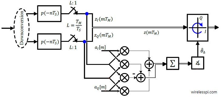
To visually comprehend the underlying signal level modifications, the Tx signal $s(t)$ in figure below consists of fast variations due to the carrier and is downconverted at the Rx by a local oscillator having a phase offset $\theta_\Delta$ with respect to the Tx. The downconverted, matched filtered and downsampled $I$ and $Q$ outputs $z_I(mT_M)$ and $z_Q(mT_M)$ are drawn next, where these are corrupted by additive noise at each stage after arriving at the Rx. Since the only distortion present is a phase offset, removing the modulation reveals $I$ and $Q$ parts of a complex number whose phase is the sought after parameter. The noise is reduced from this signal through applying a moving average filter.

Thus, the expression for the feedforward phase estimator is given by
\begin{equation*}
\hat \theta_\Delta = \measuredangle \left\{ \sum _{m=0} ^{N_P-1}a^*[m]z(mT_M)\right\}
\end{equation*}

A related estimator, except the usual difference between a four-quadrant inverse tangent and a simple inverse tangent, is
\begin{equation*}
\begin{aligned}
\hat \theta_\Delta &= \tan^{-1} \frac{\left[\sum _{m=0} ^{N_P-1}a^*[m]z(mT_M)\right]_Q}{\left[\sum _{m=0} ^{N_P-1}a^*[m]z(mT_M)\right]_I}\\
&= \tan^{-1} ~\frac{\sum \limits _{m = 0} ^{N_P-1} \Big\{ a_I[m] z_Q(mT_M) – a_Q[m] z_I(mT_M)\Big\}}{\sum \limits _{m = 0} ^{N_P-1} \Big\{a_I[m]z_I(mT_M) + a_Q[m] z_Q(mT_M)\Big\}}
\end{aligned}
\end{equation*}
where we have used the conjugate multiplication rule of complex numbers according to which $I$ and $Q$ parts of the result are given by $I\cdot I +Q\cdot Q$ and $I\cdot Q -Q\cdot I$, respectively. A block diagram for this phase estimator implementation is drawn in the the figure below, where the complex multiplication between conjugate of the known training and downsampled matched filter outputs is expanded into real operations. It is known as the maximum likelihood estimator because it is the solution of our search for finding the maximum correlation between the noisy Rx signal and its clean expected replica at the Tx.

Performance Tradeoffs

---

To see what happens in the presence of noise, consider the following in regard to the estimation equation $a^*[m]z(mT_M)$.
\begin{equation*}
\text{signal}^* \times (\text{signal} + \text{noise}) = \left(\text{signal}^*\times \text{signal}\right)~+~ \left(\text{signal}^*\times \text{noise}\right)
\end{equation*}
It is clear that due to the Rx knowledge of the training sequence $a[m]$ sent with the data, there is a single noise term and hence no noise enhancement in the estimation process. As we see later in other phase synchronization algorithms, this is not the case with non-data-aided estimators. Therefore, the phase estimation through this method renders the best performance possible.

This benefit comes at a price of increased bandwidth: assume that a data rate of $R_b$ bits/second needs to be supported on a link which translates to a symbol rate of $R_M$ $=$ $1/T_M$ symbols/second for a total of $N_D$ symbols. However, an addition of $N_P$ training symbols — and the requirement to send the same amount of bits within the same time — implies that the new symbol rate $R_{M,\text{new}}$ becomes
\begin{equation*}
R_{M,\text{new}} = R_M\left(1+\frac{N_P}{N_D}\right) \text{symbols/second}
\end{equation*}
Since the bandwidth is directly proportional to the symbol rate
\begin{equation*}
BW_{\text{QAM}} = (1+\alpha)R_M
\end{equation*}
the system needs a larger bandwidth. In other words, the power and time spent on transmitting the training sequence could have been used for sending more data: the spectral efficiency of the system is reduced by a non-negligible factor.

General Approach to Feedforward Synchronization

---

With the help from the following figure (which is an extension of the block diagram above), a general approach to feedforward phase synchronization can be constructed as follows.

1. Modulation removal: Remove the modulation from the input, i.e., the matched filter outputs.
2. Filtering: Filter the noise through summation, which in effect is a moving average filter.
3. Estimation Estimate the phase offset $\theta_\Delta$.
4. Correction Apply the correction to the input through rotating it by $-\hat \theta_\Delta$.

Other techniques to acquire phase are also available, e.g., the popular M-th power synchronizer in both feedback and feedforward settings.

This was about estimation of carrier phase offset. You can also see how a maximum likelihood estimate of a clock offset is derived.