In the context of carrier synchronization, we have discussed the Costas loop and other techniques before. Today, we discuss the significance of differential encoding and decoding for phase ambiguity resolution. Keep in mind that this topic is different than differential detection.
- In the former case, the data bits are encoded before modulation and decoded after demodulation in a differential manner. Nevertheless, the demodulation is still coherent (i.e., it requires carrier synchronization).
- In the latter case, the data symbols are detected during demodulation through differential operations, thus canceling the effect of channel phase and eliminating the need for carrier synchronization.
Let us explore this idea further.
Background
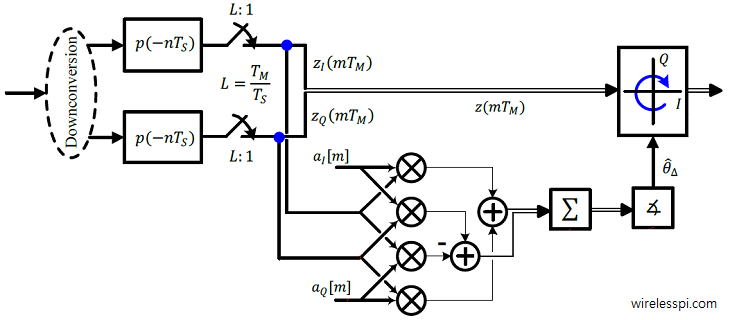
We start with the expression for a simple phase error detector that is a feedback version of the earlier feedforward phase synchronization technique.
\[
e[m] = a^*[m]z(mT_M)
\]
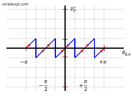
An important characteristic is the mean curve of a synchronizer (more accurately known as the S-curve) in a decision-directed scenario (i.e., when symbol decisions are employed to act as known data symbols). This is shown in the figure below.

As opposed to the S-curve of data-aided phase error detector, it crosses zero with a positive slope (and hence stable lock points) at
\[
\theta _{\Delta:e} = -\frac{\pi}{2}, 0 , +\frac{\pi}{2}, \pi
\]
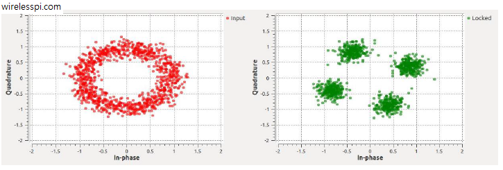
which leads to a $\pi/2$ phase ambiguity. This is indicated by arrows converging towards zeros at the positive slopes at the above locations. Consequently, the QPSK carrier phase PLL employing a decision-directed phase error detector can compensate for a carrier phase offset but it will be unknown which of the above four points it has locked to.
The resultant phase correction in subsequent symbols will contain an additional multiple of $\pi/2$ thus ruining the whole series of symbol decisions.
Similarly, a BPSK modulation has a $2\pi/2=\pi$ phase ambiguity. Therefore, the mean curve of the decision-directed phase error detector has two stable lock points, one at $0$ and the other at $\pi$.
Generalizing this observation, we conclude that a decision-directed PLL for an $M$-PSK modulation suffers from a phase ambiguity of $2\pi/M$ and offers $M$ stable locking points. There are two commonly employed methods for resolving this ambiguity:
- Unique word
- Differential encoding and decoding
We start with the unique word as it is easier to understand.
Unique Word
A unique word (UW) is just a sequence of known symbols in the data stream. After achieving phase lock, the Rx looks for this specific pattern with $0$ as well as other possible phase offsets. The phase rotation with which this pattern is found is the phase offset that needs to be corrected in the data symbols as well.
Suppose that for a BPSK modulation scheme, the UW at the start of the transmission is given by
\begin{equation*}
0~~1~~1~~0~~1
\end{equation*}
Since there are two stable lock points at $0$ and $\pi$ (which just inverts the bit), the PLL at the Rx searches for two patterns:
\begin{equation*}
0~~1~~1~~0~~1
\end{equation*}
and its rotated by $\pi$ version
\[
1~~0~~0~~1~~0
\]
If the PLL finds the former, the lock has been acquired to the actual phase and nothing needs to be done. However, if the search output indicates the latter pattern, then all of the detected data symbols need to be inverted for correct results.
Differential Encoding and Decoding
To study differential encoding and decoding, recall that we discussed the polar representation of Quadrature Amplitude Modulation (QAM) reproduced below. Usually QAM symbols are expressed through rectangular coordinates of $a_I$ and $a_Q$ through in-phase and quadrature arms. But the following representation of the same waveform in a single sinusoid is more useful here.
\begin{equation*}
\begin{aligned}
s(t) &= \sum _m \sqrt{a_I^2[m] + a_Q^2[m]} \cdot p(t-mT_M) \cdot \sqrt{2} \cos \left(2\pi F_C t+ \tan^{-1} \frac{a_Q[m]}{a_I[m]}\right) \\
&= \sum _m X[m] \cdot p(t-mT_M) \cdot \sqrt{2} \cos \left(2\pi F_Ct + \phi[m]\right)
\end{aligned}
\end{equation*}
where
\begin{align*}
X[m] &= \sqrt{a_I^2[m] + a_Q^2[m]} \\
\phi[m] &= \tan^{-1}\frac{a_Q[m]}{a_I[m]}
\end{align*}
In this polar form, we have a single sinusoid whose amplitude and phase are determined by some combination of symbols $a_I[m]$ and $a_Q[m]$ during every symbol time. For an $M$-PSK constellation, all the symbols lie on a circle and hence the amplitude $X[m]$ is constant for all symbols.
\begin{equation*}
X[m] = \text{constant}
\end{equation*}
This makes sense as only the phase is changed for a PSK modulation scheme. Let us now understand differential encoding and decoding with the help of BPSK modulation.
Encoding Process
In a regular BPSK system, the phase for the polar form $\phi[m]$ is chosen according to the incoming bit. As an example,
\begin{align*}
0 \quad \rightarrow &\quad 0 \\
1 \quad \rightarrow &\quad \pi
\end{align*}
So in the following sequence of bits $b[m]$, the mapping is shown in the table below.

It is tempting to think from the name "differential encoding" that the phase chosen for the polar form $\phi[m]$ depends on the change in bit sequence rather than the bit sequence itself. For instance, if the next bit is the same as the previous bit, the chosen phase is 0 while if the bit changes, the chosen phase is $\pi$. However, it is slightly more complicated in the sense that the change in bit sequence is with respect to the previously encoded bit, not the previous input bit. Let us see how.
Denote the encoded bit as $c[m]$ and let its starting value $c[-1]=0$. Then, we can write
\begin{equation}\label{equation-differential-encoding}
c[m] = b[m] + c[m-1] \qquad \text{mod}~2
\end{equation}
When we apply this relation to the input bit sequence $b[m]$ in the above table, we get
\begin{align*}
c[0] &= b[0] + c[-1] = 0 \\
c[1] &= b[1] + c[0] = 1 \\
c[2] &= b[2] + c[1] = 0 \\
c[3] &= b[3] + c[2] = 0 \\
\vdots
\end{align*}
The complete encoded sequence is illustrated in the figure below where the tilted arrows indicate the two terms to be summed according to the differential encoder in Eq (\ref{equation-differential-encoding}) while the downwards arrows show the results of this addition.

A block diagram for the implementation of this encoding process is drawn in the figure below.

Now we turn our attention towards the decooding process.
Decoding Process
From the differential encoding in Eq (\ref{equation-differential-encoding}), we can write the differential decoding procedure as
\begin{equation}\label{equation-differential-decoding}
\hat b[m] = \hat c[m] + \hat c[m-1] \qquad \text{mod}~2
\end{equation}
For the example sequence, assume that the PLL locks onto the incoming phase without any $\pi/2$ jump, i.e., the Rx sequence $\hat c[m]$ is the same as the Tx sequence $c[m]$. Then, applying the decoding relation in Eq (\ref{equation-differential-decoding}) with an initial value of $\hat c[-1] = 0$,
\begin{align*}
\hat b[0] &= \hat c[0] + \hat c[-1] = 0 \\
\hat b[1] &= \hat c[1] + \hat c[0] = 1 \\
\hat b[2] &= \hat c[2] + \hat c[1] = 1 \\
\hat b[3] &= \hat c[3] + \hat c[2] = 0 \\
\vdots
\end{align*}
The complete sequence $\hat b[m]$ is decoded in the figure below. Notice that it is exactly the same as the original bit sequence $b[m]$, although only the first bit can be in error for a different $c[-1] = 1$. Now if the PLL locks onto the other lock point $\pi$ as can happen in a BPSK system, the differential decoding output is still valid (except the first bit) as illustrated in this figure.

A block diagram for the implementation of this encoding process is drawn in the figure below. Keep in mind that the addition at the decoder side is actually a subtraction since they are both the same for mod-2 operations.

Concluding Remarks
One disadvantage of the differential encoding and decoding is that if one symbol is received in error and detected as $\hat c[m]$, then it will lead to two errors at the output of the final decoded sequence, as is evident from the relation in Eq (\ref{equation-differential-decoding}), one for the current bit where it participates as $\hat c[m]$ and the other for the next bit where it participates as $\hat c[m-1]$. At practical target Bit Error Rates (BER) for a well designed system, the errors are very rare for the budgeted SNR, particularly more so in consecutive symbols. We conclude that differential encoding and decoding approximately doubles the BER.