This post is written on an advanced topic mainly for practitioners and researchers in the design of wireless systems. For learning about wireless communication systems from a DSP perspective (the idea behind SDRs), I recommend you have a look at my book.
One of the main questions in the design of a wireless receiver is the interactions among the three main blocks, namely the timing recovery loop, the equalizer and the carrier recovery loop. Life would have been easy if input to any of these blocks was independent of the output from the others. That obviously is not the case. And today we explore how a symbol timing offset impacts the design of an equalizer. Keep in mind that the equalizer is a receiver block that compensates for the distortion caused by multiple signal copies arriving at the Rx in a wireless channel.
Formation of Spectral Null
Towards the end of the article on the effect of a symbol timing offset on the received signal, I presented a frequency domain view of the problem. Like me, I hope that you will also find this perspective interesting. The three scenarios drawn in the figure below are summarized next.

Let us denote the number of samples/symbol by $L$ and the timing offset by $\epsilon_\Delta$. The villain of our story is $\epsilon_\Delta$ which distorts the original signal by producing Inter-Symbol Interference (ISI).
- According the Nyquist no-ISI criterion in frequency domain, the cumulative spectrum must be a constant function of frequency from $-\infty$ to $+\infty$. Oversampling produces spectral "holes" here that cannot be filled regardless of the spectral shape. See the top subfigure above drawn for $L=2$ samples/symbol.
- As evident from the middle subfigure, sampling at $L=1$ sample/symbol and zero timing offset, the cumulative spectrum is constant and no ISI occurs.
- Even at $L=1$ sample/symbol but with a non-zero timing offset $\epsilon_\Delta$, the last subfigure above illustrates a slight dip in the cumulative spectrum. Nyquist no-ISI criterion is violated as a result. The descent gets deeper with increasing $\epsilon_\Delta$ until it reaches zero at $\epsilon_\Delta = 0.5T_M$ shown by a red line (where $T_M$ is a symbol time).
The reason for this dip, also explained in that article, is the following: for visualizing time and frequency domain transformations of a signal, remember that
\begin{equation*}
\text{Shift in one domain} \quad \rightarrow \quad \text{Multiplication by a complex sinusoid in the other domain}
\end{equation*}
Induced by the time shift $\epsilon_\Delta$, this multiplication of all the spectral replicas of the signal spectrum is drawn below in a 3D view.

Symbol-Spaced and Fractionally-Spaced Equalizers (FSE)
Due to the above analysis, one way (out of many) to classify an equalizer is with respect to the number of samples/symbol $L$ on which it operates. Naturally, the two most widely used choices are the following.
- $L=1$: This is known as a symbol-spaced or $T_M$-spaced equalizer where $T_M$ is the symbol time.
- $L>1$: This is known as a fractionally-spaced equalizer (FSE). $L$ is usually chosen as 2 to reduce the computational complexity.
Sensitivity to Timing Phase
There are two spectra shown above, one at $F=0$ and the other at $F=1/T_M$. After multiplication with frequency domain complex sinusoid $\exp(-j2\pi F \epsilon_\Delta)$, we have the expression for the cumulative spectrum sampled at $L=1$, i.e., for a symbol-spaced equalizer between $F=0$ and $F=1/T_M$.
\[
\begin{aligned}
S_{\text{Total}} &= |S(F)|^2 \exp(-j2\pi F \epsilon_\Delta) + \left|S\left(F-\frac{1}{T_M}\right)\right|^2\exp\left(-j2\pi \left(F-\frac{1}{T_M}\right)\epsilon_\Delta\right) \\
&= \exp(-j2\pi F \epsilon_\Delta)\left\{ |S(F)|^2 + \left|S\left(F-\frac{1}{T_M}\right)\right|^2\exp\left(+j2\pi \frac{\epsilon_\Delta}{T_M})\right)\right\}
\end{aligned}
\]
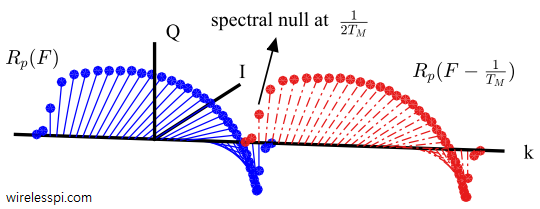
Clearly, plugging in $\epsilon_\Delta=T_M/2$ generates that $\exp(j\pi)=-1$ factor that is drawn in the last figure above. For other $\epsilon_\Delta$, the distortion is less severe but still present. A symbol-spaced equalizer is sensitive to the timing phase because inverting a spectral null enhances the noise present in that region of the spectrum.
Why is a fractionally-spaced equalizer insensitive to timing phase? To answer this question, take the example of $L=2$ samples/symbol. It is presented with a time series spaced at intervals $T_M/2$ apart. Applying the same rule of time shift in one domain and complex sinusoid in other domain, we get the spectrum between $F=0$ and $F=1/T_M$.
\[
s(mT_M/2+\epsilon_\Delta) \quad \rightarrow \quad S(F)\exp(-j2\pi F\epsilon_\Delta)
\]
because the signal has not been downsampled to $L=1$ yet. The fractionally-spaced equalizer now operates on this spectrum, compensates for the channel (and the impact of symbol timing offset) and then the aliasing due to symbol-rate sampling has any chance to add the replicas. By then, the effect of symbol timing offset is not there anymore! Representing the equalizer filter by $W(F)$, the equalized signal spectrum is given between $F=0$ and $F=1/T_M$ by
\[
S(F)W(F) + S\left(F-\frac{1}{T_M}\right)W\left(F-\frac{1}{T_M}\right)
\]
Since the equalizer filter $W(F)$ compensates for $\epsilon_\Delta$ above, the cumulative spectrum is nearly flat and satisfies Nyquist no-ISI criterion.
One might think that a symbol-rate sampling followed by a Decision Feedback Equalizer (DFE) can solve this problem due to their performance. However, remember that DFEs suffer from error propagation where one bad decision can impact decisions on future symbols too in a chain reaction. To cancel the spectral null, a relatively long impulse response in the feedback filter is required with large magnitude coefficients. Such a filter suffers from an even higher level of error propagation.
References
[1] J. Spilker, Digital Communication by Satellite, Prentice Hall, 1977.