What is a Symbol Timing Offset and How It Distorts the Rx Signal

Timing synchronization is one of the most fascinating topics in the field of digital communications. On the bright side, numerous scientists have contributed towards its body of knowledge due to its crucial role in the successful implementation of communication and storage systems. On the not-so-bright side, this knowledge has grown to an extent that it has also become the least understood and puzzling topic in the grand scheme of things. My objective in this article is to simplify the problem in a clear and intelligible manner, and also refer to some of the most widely used solutions within the explanation.

Symbol timing synchronization is also known as symbol timing recovery, clock synchronization and clock recovery. The word symbol is very important here because time synchronization is a broader term that can refer to other kinds of synchronization as well such as network synchronization among computer or microcontroller clocks, packet synchronization in telecommunication systems, and so on.

Symbol Timing Offset

---

One of the foremost tasks of a digital Rx is to determine the starting point of the useful component in a sampled Rx signal, as many of its initial samples are noise only. It is the job of a frame synchronization unit to determine symbol number $1$ in the Rx sequence. Once the frame synchronization is achieved, the job of the symbol timing synchronization block is to establish the optimal sampling instant within a symbol. The Rx needs to sample the received sequence every $T_M$ seconds at exactly these instants when the eye opening is maximum (points of no ISI from the neighbouring symbols). However, the peak sample at the end of the matched filter output for each symbol duration is not known in advance at the Rx. This is illustrated in Figure below for a signal sampled at $2$ samples/symbol.

In the top part of the figure, a Rx sampled the signal at exactly $2$ samples/symbol, one of which coincides (fortunately) with the optimal sampling instants (integer multiples of $T_M$) shown as white circles. In reality, this peak sample does not coincide at all with a generated sample at the Rx. This is because the ADC just samples the incoming continuous waveform without any information about the symbol boundaries. This is illustrated in the bottom part of this figure where $\varepsilon_\Delta$ is the timing phase offset by which the Rx clock is misaligned in reference to the Tx clock. An efficient mechanism needs to be invoked to construct the missing samples at the exact symbol boundaries, shown as black and white dots here.

As a first solution, it is possible to transmit both the data and the clock in a Tx waveform (for example, the data at the $I$ channel and the clock signal at the $Q$ channel in a QAM waveform) so that the Rx can produce the samples that are exactly aligned with the symbol boundaries according to the Tx. However, it requires sacrificing a part of the power and bandwidth because the resources dedicated to send the clock signal could be used to send more data as well. To avoid wasting the precious resources in this context, techniques to extract the Tx clock from the noisy received data waveform itself need to be devised.

In the days of analog signal processing and the early years of digital processing, symbol timing synchronization was accomplished by generating a clock signal that is aligned (in both phase and frequency) with the clock used to generate the data at the Tx. This was a Voltage Controlled Clock (VCC) driven by a filtered timing error detector output, just like a Voltage Controlled Oscillator (VCO) driven by a filtered phase error detector output in a Phase Locked Loop (PLL). After the proliferation of digital signal processing, this definition is not that helpful due to the fixed rate sampling and interpolation. Instead, an all-digital timing locked loop is now employed for this purpose that utilized a range of timing error detectors such as early-late, zero-crossing and Mueller and Muller techniques.

In light of the above discussion, the goal of digital timing synchronization is to produce $L$ samples per symbol at the matched filter output such that one of those samples is aligned with the maximum eye opening. As usual, the effect of a symbol timing offset $\varepsilon_\Delta$ can be visualized in both time and frequency domains. In this post, I will describe this effect in time domain and leave the frequency domain explanation for some other day.

Time Domain View

---

To understand the role of a symbol timing mismatch in time domain, we begin with an $M$-PAM signal as
\begin{equation*}
s(t) = \sum _{i} a[i] p(t-iT_M)
\end{equation*}
where $a[i]$ is the $i^{th}$ data symbol, $p(t)$ is a square-root Nyquist pulse with support $-LG \le t \le LG$ samples, $L$ is the number of samples/symbol, $G$ is the group delay or one-sided pulse length in symbols and $T_M$ is the symbol time. Ignoring every other distortion at the Rx except a Symbol Timing Offset (STO) $\varepsilon_\Delta$, the received signal $r(t)$ is given as
\begin{equation}\label{eqTimingSyncRxSignal}
r(t) = \sum _{i} a[i] p(t-iT_M-\varepsilon_\Delta)
\end{equation}
In the above equation, the range of $\varepsilon_\Delta$ is defined as a fractional value within a symbol interval $T_M$.
\begin{equation*}
-0.5T_M \le \varepsilon_\Delta \le +0.5T_M
\end{equation*}
which is why it is known as a timing phase. Note that we are defining the symbol timing offset $\varepsilon_\Delta$ in units of the symbol time $T_M$. When there is a need of a normalized Symbol Timing Offset (nSTO) in an expression, we will use the notation $\varepsilon_0$ which implicitly carries a factor of $T_M$ within itself in terms of a percentage.
\begin{equation*}
-0.5 \le \varepsilon_0 = \frac{\varepsilon_\Delta}{T_M} \le +0.5
\end{equation*}

Now, we examine what happens when the Rx samples this signal in Eq (\ref{eqTimingSyncRxSignal}) through an ADC operating at a rate of $F_S=1/T_S$ samples/second, the output of which is
\begin{equation*}
r(nT_S) = \sum _{i} a[i] p(nT_S-iT_M-\varepsilon_\Delta)
\end{equation*}
This signal is input to a matched filter $h(nT_S) = p(-nT_S)$.
\begin{align}
z(nT_S) &= \Big\{ \sum \limits _i a[i] p(nT_S – iT_M-\varepsilon_\Delta)\Big\} * p(-nT_S) \nonumber\\
&= \sum \limits _i a[i] r_p(nT_S -iT_M -\varepsilon_\Delta) \label{eqTimingSyncMFoutput}
\end{align}
where $r_p(nT_S)$ comes into play from the definition of the pulse auto-correlation. This is plotted in Figure below for a $25\%$ timing offset where the sampling is not being performed at optimal instants. We will next zoom into this figure for a detailed discussion.

To generate symbol decisions, $T_M$-spaced samples of the matched filter output are required at $n = mL = mT_M/T_S$. Downsampling the matched filter output generates
\begin{align}
z(mT_M) &= z(nT_S) \bigg| _{n = mL = mT_M/T_S} \nonumber \\
&= \sum \limits _i a[i] r_p(mT_M – iT_M-\varepsilon_\Delta) = \sum \limits _i a[i] r_p\Big[( m-i)T_M-\varepsilon_\Delta\Big] \nonumber \\
&= \underbrace{a[m] r_p (-\varepsilon_\Delta)}_{\text{Term 1}} + \underbrace{\sum \limits _{i \neq m} a[i] r_p\Big[(m-i)T_M -\varepsilon_\Delta\Big]}_{\text{Term 2}} \label{eqTimingSyncSymbolTimingISI}
\end{align}

The above equation reveals that the optimal samples at the matched filter output can be broken into the following two terms:

Term 1: Desired Signal is given by $a[m] r_p (-\varepsilon_\Delta)$. From the details of a pulse shaping filter, we know that the maximum output of a Nyquist pulse auto-correlation is $1$ and it is delivered at instant $0$. Therefore, the effect of $r_p (-\varepsilon_\Delta)$ is to reduce the desired symbol estimate $a[m]$ by an amount proportional to the Symbol Timing Offset (STO) $\varepsilon_\Delta$.

Term 2: Inter-Symbol Interference (ISI) is the accumulation of contributions from all other symbols in the neighborhood of the current symbol, up to the pulse group delay. This contribution, again, depends on the timing offset $\varepsilon_\Delta$.

---

By zooming in on the terms $i=m-1$, $i=m$ and $i=m+1$, we can also write Eq (\ref{eqTimingSyncSymbolTimingISI}) as
\begin{align*}
z(mT_M) &= a[m] r_p (-\varepsilon_\Delta) + \\
&\hspace{.5in} \cdots + a[m-1] r_p(T_M -\varepsilon_\Delta) + a[m+1] r_p(-T_M -\varepsilon_\Delta) + \cdots
\end{align*}
The consequences of the above equation can be observed by the shaded region in Figure below which is a zoomed in version of the above figure. Here,

• the current symbol has reduced in amplitude, and
• adjacent two ISI terms can be seen as interfering with the current symbol estimate.

The STO here is $0.25T_M$ which for a sample rate of $4/T_M$ means an offset of $1$ sample. I recommend you to carefully look at this figure to understand the interference from the other symbols for an incorrect sampling instant.

The vertical dashed lines illustrate the actual symbol boundaries which is where the samples should be taken. However, due to the timing offset, the contributions from $a[m-1]$ and $a[m+1]$ are not zero. The amount of their interference is dictated by this offset while the sign is governed by the modulating data values.

Eye Diagram and Scatter Plot

---

When many such scaled pulse shapes are added together to form a Pulse Amplitude Modulation (PAM) waveform, we can see the behavior more clearly through sampling an eye diagram for different timing offsets. Figure below illustrates an example for three different $\varepsilon_\Delta$:
\begin{equation*}
\varepsilon_\Delta = 0, ~0.25T_M ~~\text{and}~ -0.5T_M
\end{equation*}
which we discuss below. At a rate of $L$ samples/symbol, these values of $\varepsilon_\Delta$ correspond to $0$, $L/4$ and $-L/2$ samples, respectively. Obviously, a symbol timing offset can fall anywhere between the samples as well. In this figure, pay close attention to the solid and dotted arrows as they reveal different characteristics for the symbol timing.

$\varepsilon_\Delta=0$

---

This case corresponds to the perfect symbol estimates at the center of the eye diagram, which is at the end of the symbol interval $T_M$ in the actual matched filter output (recall that an eye diagram is drawn within an interval $-0.5T_M \le t \le +0.5T_M$). This is where the eye opening on average is at its maximum and no ISI from the neighboring symbols distorts this optimal sample. A timing error samples the eye diagram at some other instant.

$\varepsilon_\Delta=-0.5T_M$

---

This scenario corresponds to the maximum symbol timing offset a digital system can have. In the eye diagram, it is the left edge of the interval, as drawn in Figure below, or the middle of the symbol interval $T_M$ in an actual symbol stream. Any $\varepsilon_\Delta$ lesser than that will come around from the right side of the eye diagram (and the integer $1$ will be deleted from the integer output of the frame synchronization block). For example, an offset of $\varepsilon_\Delta=-0.6T_M$ will appear as $+0.4T_M$. Without any aid from the frame synchronization block, we would have encountered a cycle slip.

In an earlier post, it was shown that tracing a single transition in an eye diagram gives information about $3$ symbols: Past, NOW and Future. For this reason, a different sequence of $+1$s and $-1$s carves a different path on the eye diagram. This is the reason an eye diagram has different traces coming to the same $+1$ value: coming from top indicates the previous symbol being $+1$ and middle for previous symbol being $-1$. The traces leaving a $+1$ value follow a similar logic: leaving towards the top indicates the next symbol being $+1$ and middle for next symbol being $-1$.

But in the figure above, another three distinct routes can be identified at the bottom of $Q$ Eye from a $-1$ to a $-1$ transition. This is due to the sequence values coming before the previous symbol. So a $+1$, $-1$, $-1$ will follow a slightly different path as compared to a $-1$, $-1$, $-1$, and so on. Considering a similar contribution arriving from the $I$ branch at the top, middle and bottom, a total of $3\times 3=9$ modulation points for each constellation point arise in the scatter plot.

Finally, notice that the magnitude of these points in the scatter plot tends to be greater than the ideal constellation point denoted by a star. This can be recognized by looking at the eye diagram at $-0.5T_M$ where two out of three paths have a higher magnitude than the ideal point at the sampling instant.

$\varepsilon_\Delta=+0.25T_M$

---

The final example corresponds to sampling at the quarter symbol interval on the right half of the eye diagram. Two distinct patterns can be distinguished in the scatter plot, which correspond to the eye diagram, say for example, out of a $+1$ value, those heading towards the top and those heading towards the middle. A total of $4=2\times 2$ distinct regions for each ideal constellation point in the scatter plot arise due to a similar contribution from $I$ arm (indicated by the ellipses and the arrows).

For this region, scatter plot shows lesser magnitude on average than the ideal constellation point. This is again evident from the corresponding eye diagram.

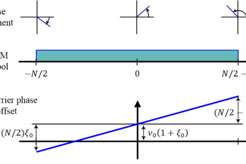
Analogy Between the Carrier Phase and Symbol Timing Offsets

---

The above study tells us an interesting analogy between the carrier phase offset and symbol timing offset. Just like the phase is defined between $-\pi$ to $+\pi$ and everything else is wrapped around, a symbol timing offset is defined between $-0.5T_M$ and $+0.5T_M$ and everything else wraps around. On that account, $T_M$ is to symbol timing what $2\pi$ is to carrier phase. This analogy is documented in the table below.

Until now, the explanation rotated around the time domain. To see what effect it has in the frequency domain, first consider a square-root Nyquist pulse shaping filter alone instead of a shaped data sequence. Since this pulse shape is a real and even signal in time domain, it is also a real and even signal in frequency domain. Recall from the article on effect of time shift in frequency domain that a right shift of $n_0$ samples in a time series changes the phase of its DFT by $-2\pi (k/N) n_0$ for each $k$.

\begin{equation*}
\begin{aligned}
\text{Time shift} \quad s[(n-n_0) \:\text{mod}\: N] \quad &\rightarrow \quad -2\pi \frac{k}{N} n_0 \quad \text{Phase shift} \\
&\text{for each}~ k = -N/2, \cdots,-1,0,1,\cdots,N/2-1
\end{aligned}
\end{equation*}
For a continuous-time case, this is given by
\begin{equation}\label{eqTimingSyncDelayPhase}
\text{Time shift} \quad s(t-\epsilon_\Delta) \quad \rightarrow \quad -2\pi F \epsilon_\Delta \quad \text{Phase shift}
\end{equation}
With a fixed $\epsilon_\Delta$ and frequency $F$ as the variable, the right hand side above becomes a complex sinusoid. We conclude that a time shift of $\epsilon_\Delta$ represents multiplication in frequency domain of the signal with a complex sinusoid of inverse period $\epsilon_\Delta$ (inverse period by definition is frequency; however, we are already in frequency domain and hence this expression).

\begin{equation*}
\text{Shift in one domain} \quad \rightarrow \quad \text{Multiplication by a complex sinusoid in the other domain}
\end{equation*}

Another way to look at this is as follows: in time domain, a signal mixed (multiplied) with a complex sinusoid of a certain frequency causes a spectral shift in frequency domain (this is how spectrum is shared worldwide, e.g., a garage door opener works at a frequency of around $400$ MHz and our WiFi modem at $2.4$ GHz). Owing to time frequency duality, a shift in time domain implies multiplication with a complex sinusoid in frequency domain.

Armed with this knowledge, it is easy to see that a pulse shaping filter gets rotated by $-2\pi F \epsilon_\Delta$ in frequency domain and the resampling must compensate for this rotation by adjusting its phases in the opposite direction. Next, we extend this concept in relation to the sample rate $F_S$. This is because the final decision device (threshold detector) operates at a symbol rate $R_M=1/T_M$, i.e., $T_M$-spaced samples of the matched filter output are required to generate symbol decisions and our final target is to investigate what happens when we directly sample the signal at $F_S=1/T_M$. As before, the pulse shape suffices to study this effect and a whole modulated sequence is not needed.

$L=2$ samples/symbol

---

For this purpose, we start with the sample rate $F_S$ equal to $L$ samples/symbol where $L >= 2$. Figure below draws the spectrum of a Raised Cosine pulse with excess bandwidth $\alpha=0.5$ which is sampled at $F_S=2/T_M$, or $2$ samples/symbol. The replicas arising as a result of sampling are naturally $2/T_M$ apart and hence produce spectral “holes” here that cannot be filled regardless of the spectral shape. Recall from Nyquist no-ISI criterion in frequency domain here that the cumulative spectrum must be a constant function of frequency from $-\infty$ to $+\infty$.
$$\begin{equation}
\begin{aligned}
\sum \limits _{i=-\infty} ^{\infty} R_p(F + \frac{i}{T_M}) &= \cdots + R_p(F + \frac{1}{T_M}) + \\
&\hspace{0.5in} R_p(F) + R_p(F – \frac{1}{T_M}) + \cdots = T_M
\end{aligned}
\end{equation}\label{eqTimingSyncNyquistnoISI}$$

Thus, ISI can only be avoided at $L=1$ sample/symbol which we explore next.

$L=1$ sample/symbol, $\epsilon_\Delta=0$

---

Now we draw the same spectrum but for a sample rate of $F_S=1/T_M$, or $1$ sample/symbol but no timing offset in the figure below. The cumulative spectrum is flat because there is no rotation in frequency domain arising from $\epsilon_\Delta$. Thus, Nyquist no-ISI criterion is satisfied and the resulting symbol-spaced samples in time domain will exhibit no ISI.

What happens when there is a timing offset present? This is what we discuss next.

$L=$1 sample/symbol, $\epsilon_\Delta\neq 0$

---

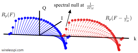
Finally, for $F_S=1/T_M$, or $L=1$ sample/symbol, but with a timing offset of $\epsilon_\Delta=0.2T_M$, the blue line in the figure below illustrates a slight dip in the cumulative spectrum. Nyquist no-ISI criterion is violated as a result. The descent gets deeper with increasing $\epsilon_\Delta$ until it reaches zero at $\epsilon_\Delta = 0.5T_M$ shown by a red line. We conclude that a timing shift of $\epsilon_\Delta$ puts the spectrum of the pulse auto-correlation $R_p(F)$ and its $1/T_M$ shifted version $R_p(F\pm 1/T_M)$ out of phase. As a consequence, the spectrum reduces in amplitude over the portion of frequency overlap, developing into a notch as $\epsilon_\Delta$ approaches $0.5T_M$.

Now we draw all three spectra discussed above together to have a clearer comparison.

Spectral Cancellation

---

The figure below compares the spectral illustrations described above.

Mathematically, we can see why there is a reduction in spectral amplitude around the frequency $1/2T_M$. From Eq (\ref{eqTimingSyncNyquistnoISI}), the spectrum between $0$ and $1/T_M$ after sampling is given by
\begin{equation*}
R_p(F) + R_p\left(F-\frac{1}{T_M}\right) \qquad 0 \le F \le \frac{1}{T_M}
\end{equation*}

Since the pulse is real and even, the pulse auto-correlation $r_p(nT_S)$ has a real and even Fourier Transform $R_p(F)$ with zero phase. Then, a delay of $\epsilon_\Delta$ injects the following phase shift according to Eq (\ref{eqTimingSyncDelayPhase}).
\begin{equation}\label{eqTimingSyncSpectralReplicaShift1}
\text{Phase shift in}~ R_p(F) = -2\pi F \epsilon_\Delta
\end{equation}

However, the phase shift in its replica at $1/T_M$ is
$$\begin{equation}
\begin{aligned}
\text{Phase shift in}~R_p\left(F-\frac{1}{T_M}\right) &= -2\pi \left(F-\frac{1}{T_M}\right) \epsilon_\Delta \\
&= -2\pi F\epsilon_\Delta + 2\pi \frac{1}{T_M}\epsilon_\Delta
\end{aligned}
\end{equation}\label{eqTimingSyncSpectralReplicaShift2}$$

The term $2\pi (1/T_M) \epsilon_\Delta$ for $\epsilon_\Delta=0.5T_M$ becomes
\begin{equation*}
2\pi \frac{1}{T_M} \cdot 0.5T_M = \pi
\end{equation*}

Hence, Eq (\ref{eqTimingSyncSpectralReplicaShift2}) yields
\begin{equation*}
\text{Phase shift in}~R_p\left(F-\frac{1}{T_M}\right) = – 2\pi F\epsilon_\Delta + \pi
\end{equation*}

which is exactly opposite to that of the original spectrum $R_p(F)$, see Eq (\ref{eqTimingSyncSpectralReplicaShift1}). A phase shift of $\pi$ is the same as multiplication by $-1$. Hence, the cumulative spectrum \bbf{for $\epsilon_\Delta=0.5T_M$} is given by

This subtraction of spectral components reduces their amplitudes. Particularly, at $F = 1/2T_M$, the phase shift of $R_p(F)$ is
\begin{align*}
– 2\pi F \epsilon_\Delta = – 2\pi \frac{1}{2T_M}\cdot 0.5 T_M = – \frac{\pi}{2}
\end{align*}
while the phase shift of $R_p(F-1/T_M)$ is
\begin{align*}
– 2\pi F \epsilon_\Delta + \pi = – 2\pi \frac{1}{2T_M}\cdot 0.5 T_M + \pi = – \frac{\pi}{2} +\pi = +\frac{\pi}{2}
\end{align*}
This $\mp \pi/2$ phase relationship is more clearly drawn below for a small excess bandwidth $\alpha=0.1$ for clarity. Their addition generates the spectral null you saw in the 3rd figure above for a case of $\epsilon_\Delta=0.5T_M$. Not drawn in this figure is the alias at the negative side for clear illustration.

Not surprisingly, this frequency $1/2T_M$ plays a central role in most timing synchronization algorithms.

Concluding Remarks

---

• Notice here that more spectral cancellation happens for large excess bandwidths and less cancellation for small excess bandwidths. Due to this reason, symbol timing strategies operating at $L=1$ sample/symbol (e.g., Mueller and Muller algorithm) usually exhibit better performance for low excess bandwidths.
• See this article for an intuitive explanation of how excess bandwidth impacts the performance of timing synchronization.
• Feedforward timing synchronization schemes are also possible, such as a digital filter and square timing acquisition.
• A symbol-spaced equalizer and a fractionally-spaced equalizer have different sensitivities to the symbol timing offset.

---