Effect of Time Shift in Frequency Domain

Children usually ask questions like “How many hours have passed?” And they have no idea about the start time to be taken as a reference.

Just like the zero of a measuring tape, a zero reference for time plays a crucial role in analyzing the signal behaviour in time and frequency domains. Until now, we assumed that reference time $0$ coincides with the start of a sine and a cosine wave to understand the frequency domain. Later, we will deal with symbol timing synchronization problem in single-carrier systems and carrier frequency synchronization problem in multicarrier systems, both of which address the problem of finding this reference to prevent signal distortion. To solve those problems, we study the signals with arbitrary time shifts and want to know their effects on frequency domain behaviour.

To begin with, let us shift a cosine signal by $T/4$ to the right where $T$ is its time period $T=1/F$.
\begin{align*}
\cos2\pi F\left(t-\frac{T}{4}\right) &= \cos \left(2\pi Ft -2\pi F\frac{T}{4}\right) = \cos \left(2\pi Ft – \frac{\pi}{2}\right) = \sin 2\pi Ft
\end{align*}
where a time shift of $-T/4$ is seen to impart a phase shift of $-\pi/2$ in frequency domain. This makes sense because if a full period $T$ of the two complex sinusoids summing up in time domain to produce a cosine spans $360^\circ$, then a shift of $-1/4$ of $360^{\circ}$ is $-90^{\circ}$. This is illustrated in Figure below.

This is why you often see a phase description for a real cosine wave as in Figure below. Taken as the reference times, these phases are due to the orientation of the two complex sinusoids in frequency $IQ$-plane and present a more interesting view (although simple trigonometric formulas like $\cos0=1$, $\cos \pi/2=0$ can also be applied to see this phase relationship).

Now evaluate a discrete-time complex sinusoid for a general time shift of $n_0$ samples. Since this is in context of the DFT, the shift here is circular even if not explicitly stated.
\begin{align*}
\cos 2\pi \frac{k}{N} \left(n + n_0\right) = \cos \left( 2\pi \frac{k}{N} n + 2\pi \frac{k}{N} n_0 \right) \\
\sin 2\pi \frac{k}{N} \left(n + n_0\right) = \sin \left( 2\pi \frac{k}{N} n + 2\pi \frac{k}{N} n_0 \right) \\
\end{align*}
There are two ways to look into this expression.

Effect of Time Shift on DFT – Magnitude and Phase

This complex sinusoid can be seen to undergo a phase shift equal to $2\pi(k/N)n_0$. Since the DFT of a signal is just a combination of $N$ such complex sinusoids with distinct values of $k/N$, the phase of the DFT considering each $k$ becomes a linear function of discrete frequency $k/N$.
\begin{equation*}
\text{phase shift} = 2\pi \frac{k}{N}n_0 = \text{constant}\cdot \frac{k}{N}
\end{equation*}
where the constant term, or slope, depends on the circular time shift $n_0$. Also, the bigger the index $k$, the larger the phase shift is. Such a phase plot is drawn in Figure below for a positive $n_0$.

In conclusion, the DFT of $\tilde s[n]$ $=$ $s[(n+n_0) \:\text{mod}\: N]$ has its magnitude unchanged. However its phase is rotated by $2\pi (k/N) n_0$ for each $k$. We denote the rotated DFT by $\widetilde{S}[k]$.
\begin{equation}\label{eqIntroductionDFTShiftMagnitudePhase}
\begin{aligned}
|\widetilde{S}[k]| &= |S[k]| \\
\measuredangle \widetilde{S}[k] &= \measuredangle S[k] + 2\pi \frac{k}{N} n_0
\end{aligned}
\end{equation}
We can summarize the above result as

This is the view mostly taken while describing the effect of a time shift and it serves well for the mathematical purpose. In my opinion, the effect of a time shift can be better visualized through $IQ$ plots that follow next.

Effect of Time Shift on DFT – $I$ and $Q$

A more interesting view comes from focusing on $I$ and $Q$ samples of the frequency domain. Let us shift an impulse signal $\delta[n]$ by $n_0$. Plugging $s[n]$ $=$ $s_I[n]$ $=$ $\delta[(n+n_0) \:\text{mod}\: N]$ in the DFT definition and using the fact that it is $1$ at $n=-n_0$ and $0$ everywhere else,
\begin{align*}
S_I[k]\: &= \sum \limits _{n=0} ^{N-1} \delta[n+n_0]\cos 2\pi\frac{k}{N}n = \cos 2\pi\frac{k}{N}n_0\\
S_Q[k] &= \sum \limits _{n=0} ^{N-1}- \delta[n+n_0]\sin 2\pi\frac{k}{N}n = \sin 2\pi\frac{k}{N}n_0
\end{align*}

for each $k$ where we have used $\cos(-A)=\cos A$ and $-\sin(-A)=\sin A$. Observe that the above expression represents a frequency domain complex sinusoid! Let us explore it with the help of an example.

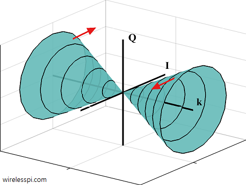
To understand this frequency domain complex sinusoid, recall that a time domain complex sinusoid rotating at frequency $F$ was shown to generate a helix in time $IQ$-plane. Such a complex sinusoid has a frequency domain representation that consists of a single impulse at $+F$. This is how we defined each `tick’ on the frequency axis.
\begin{equation*}
\text{Time domain complex sinusoid} \quad \leftarrow\rightarrow \quad \text{Frequency domain impulse}
\end{equation*}
Since time and frequency are dual of each other, the time domain impulse in this example drawn in Figure above must have a corresponding frequency domain complex sinusoid.
\begin{equation}\label{eqIntroductionTimeImpulseFreqHelix}
\text{Time domain impulse} \quad \leftarrow\rightarrow \quad \text{Frequency domain complex sinusoid}
\end{equation}
And that is exactly what a phase shift of $2\pi (k/N) n_0$ represents as a function of $k$. This is shown for $n_0=-1$ in Figure below, a redrawn version of the bottom right of Figure above. The important point here is that the frequency index $k$ is the variable of this frequency domain complex sinusoid. On the other hand, time shift $n_0$ is an inverse period of this sinusoid and plays the role similar to frequency $F$ in the expression $2\pi Ft$.

\begin{equation*}
\text{phase shift} = 2\pi (n_0) \frac{k}{N} = 2\pi \big(\text{inverse period}\big) \frac{k}{N}
\end{equation*}

Now let us apply the time shift to a time domain complex sinusoid. Using the identities $\cos (A+B)$ $=$ $\cos A \cos B$ $-$ $\sin A \sin B$ and $\sin (A+B)$ $=$ $\sin A$ $\cos B$ $+$ $\cos A \sin B$,
\begin{align*}
\cos 2\pi \frac{k}{N} \left(n + n_0\right) &= \cos 2\pi \frac{k}{N} n \cdot \cos 2\pi \frac{k}{N} n_0 – \\
&\hspace{1.4in}\sin 2\pi \frac{k}{N} n \cdot \sin 2\pi \frac{k}{N} n_0 \\
\sin 2\pi \frac{k}{N} \left(n + n_0\right) &= \sin 2\pi \frac{k}{N} n \cdot \cos 2\pi \frac{k}{N} n_0 + \\
&\hspace{1.4in}\cos 2\pi \frac{k}{N} n \cdot \sin 2\pi \frac{k}{N} n_0
\end{align*}

From the multiplication rule of complex numbers $I \cdot I$ $-$ $Q \cdot Q$ and $Q \cdot I$ $+$ $I \cdot Q$, we can see that in frequency domain, our original complex sinusoid is again being multiplied with another frequency domain complex sinusoid given by
\begin{align*}
V_I[n]\: &= \cos 2\pi\frac{k}{N}n_0\\
V_Q[n] &= \sin 2\pi \frac{k}{N}n_0
\end{align*}

Finally, what happens when $N$ analysis frequencies are present (the complex sinusoids that form the DFT)? Extending the same concept proved above and noting that a DFT is a combination of $N$ complex sinusoids, the DFT of $\tilde s[n]$ $=$ $s[(n+n_0) \:\text{mod}\: N]$ is given by the following expression which is also straightforward to prove through DFT definition.

i.e., the DFT is multiplied with a frequency domain complex sinusoid as $n_0$ is fixed and $k$ varies (in terms of complex signals, this expression is written for a signal $s(t)$ as $s(t-t_0)$ $\rightarrow$ $S(F)\cdot \exp(-j2\pi Ft_0)$).

This is the most important relation to understand for visualizing time and frequency domain transformations of a signal and we summarize it as
\begin{equation*}
\text{Shift in one domain} \quad \rightarrow \quad \text{Multiplication by a complex sinusoid in the other domain}
\end{equation*}

The magnitude and direction of rotation for these frequencies is symbolically shown for a positive $n_0$ in Figure below.

Another way of understanding the above relation $s(t-t_0)$ $\rightarrow$ $S(F)\cdot \exp(-j2\pi Ft_0)$) is that a simple time shift $t_0$ results in a linear phase response $-2\pi Ft_0$. This is very important in many filter design applications.

Significance of Linear Phase

As far as a linear phase is concerned, it preserves the waveform shape due to the following reason. A simple delay ensures the waveform integrity in time domain. When the signal is composed of constituent sinusoids, all of them need to be delayed by the same time (and not by the same phase). Intuitively, if sinusoids with different frequencies get delayed by the same number of samples, then they naturally end up with different phases at the end of that common duration, as illustrated in Figure below. However, each of those phases is the common delay multiplied with that frequency. The overall sum of the sinusoids with different frequencies still remains the same.

On the other hand, if the phase is non-linear, then the delay introduced in the waveform is not proportional to the frequency, thus different constituent sinusoids get delayed by varying amounts of time which distorts the signal shape, commonly known as phase distortion. In wireless communications, the target is to maintain a linear phase of the signal for proper detection.

True insights can only be developed through grasping the implications of phase rotations as well as time and frequency domain complex sinusoids.