FMCW Radar Part 2 – Velocity, Angle and Radar Data Cube

In Part 1 of FMCW radar series, we described how a radar estimates the range of one or more stationary targets. In Part 2, we talk about estimating the velocities of several moving targets and their directions through forming a structure known as the radar cube. Part 3 presents system design guidelines for an FMCW radar.

---

In a wonderful 1991 paper "Wireless Digital Communication: A View Based on Three Lessons Learned", Andrew Viterbi summarizes the Shannon theory for digital communications in the form of 3 lessons, the first of which was the following.

"Never discard information prematurely that may be useful in making a decision until after all decisions related to that information have been completed."

The applications of this lesson lead to soft decision decoding in error control codes and maximum-likelihood sequence estimation in high-rate wireline modems. In this article, we utilize the same principle and explore how much information can be extracted from a simple echo returning from a target.

Background

---

A CW radar measures the velocity of an object by measuring the change in frequency. In theory, an FMCW radar can measure the velocity of a target in the same way. A fancy equation can be derived that detects the change in chirp rate and the change in frequency to yield the velocity. However, this a complicated solution and requires far more data than the simple technique practically deployed and detailed in this article.

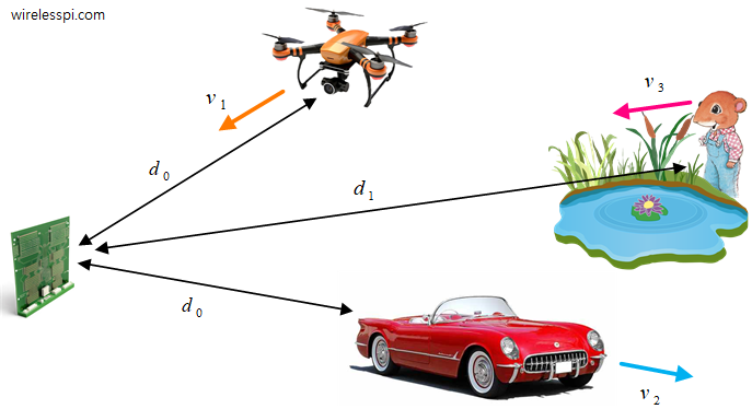
Consider again the two vehicles as in Part 1 and shown in the figure below. During the investigation on a CW radar, we showed how the change in phase contains the range information while the change in frequency (Doppler) carries the speed information.

The problem discovered with a CW radar was that the unique range can only be determined within the unambiguous span of $\pm \pi$. An FMCW radar overcomes this obstacle by introducing modulation that helps extract the range through beat frequency estimation.

With this knowledge, what do you think happens when the stationary vehicle in the above figure starts moving at a velocity $v$? Since the movement causes a Doppler frequency $f_d$ of its own, the beat frequency $f_b$ will shift by an amount equal to $f_d$. This is illustrated in a figure below for both positive and negative Doppler scenarios.

Let us focus on the positive $f_d$ case only as in the left figure. The beat frequency here is given by
\begin{equation}\label{equation-up-chirp}
f_{b,up} = f_b ~- f_d
\end{equation}

It has become impossible to separate the Doppler frequency from the beat frequency through the same technique because there are two unknowns in one equation.

Next, we describe one possible solution to this problem along with its limitations.

Using the Triangular Chirp

---

The issue of two unknowns in one expression can be solved through searching for another equation involving both variables. There are two pointers to guide us here.

• Recall from Part 1 the principle of changing the signal if the target is not moving. Now when the target is moving, how can the signal be changed again such that it provides a second equation to estimate both the range and the speed?
• In a time of flight ranging system, a backward communication is set up to provide a second equation for simultaneous estimation of delay and phase offset. This results in one parameter (the phase offset) appearing with an opposite sign.

Taking hints from the above observations, the waveform can be modified such that a linearly decreasing frequency (the down-chirp) follows a linearly increasing frequency (the up-chirp). This results in an overall triangular chirp as shown in the figure below.

These upchirps and downchirps look a lot like a year of sunrises. The figure below shows the sunrises taken in Edmonton, Alberta, Canada each month with camera facing the east. In the month of June at the northern hemisphere, the sun starts moving to the right (southward) until the winter arrives in December and then returns to the left (northward) with the arriving summer in June.

Sunrise over 12 months at Edmonton, Alberta, Canada. Image Credit/Copyright: Luca Vanzella

The benefit of the down-chirp is the appearance of one parameter (the Doppler frequency) with an opposite sign, as compared to Eq (\ref{equation-up-chirp}).
\begin{equation}\label{equation-down-chirp}
f_{b,down} = f_b ~+ f_d
\end{equation}

The estimation procedure can now be detailed in the following steps.

• The frequencies $f_{b,up}$ and $f_{b,down}$ in Eq (\ref{equation-up-chirp}) and Eq (\ref{equation-down-chirp}), respectively, belong to simple sinusoids embedded in noise at the mixer output. They can be estimated through any of the several techniques available for this purpose, see the frequency synchronization chapter for some examples.
• The beat frequency $f_b$ was linked to the range $d_0$ through this Equation in Part 1.
  \[
  f_b = \mu\frac{2d_0}{c} = \frac{f_{b,down} + f_{b,up}}{2}
  \]

  where we have used Eq (\ref{equation-up-chirp}) and Eq (\ref{equation-down-chirp}) to derive the right hand side.

• On a similar note, we also saw that the Doppler frequency $f_d$ is related to the velocity $v$ through this Equation in Part 1 as
  \[
  f_d = \frac{2v}{\lambda} = \frac{f_{b,down} – f_{b,up}}{2}
  \]

• All this leads to two unknowns, range $d_0$ and velocity $v$, in two equations that can be solved as
  \[
  \begin{aligned}
  d_0 &= \frac{f_{b,down} + f_{b,up}}{4}\cdot \frac{c}{\mu} \\
  v &= \frac{f_{b,down} – f_{b,up}}{4}\cdot \lambda
  \end{aligned}
  \]

The major theme of this solution is that two different chirp rates $+\mu$ and $-\mu$ are employed and hence it works with range and velocity of one moving target only. If there are multiple targets, then two equations are inadequate for determining their ranges and velocities. Moreover, ghost targets appear from intersections of lines belonging to, say, first and second target, which cause ambiguity in range-velocity map.

Generalizing the above idea, we can keep changing the signal through incorporating multiple chirp rates in each sweep depending on the expected number of targets. In fact, some researchers have proposed and implemented this idea. However, it results in a significantly complicated radar design. Instead, a simple solution is described below that relies on the fact that the change in Doppler frequency is negligible from one chirp to the next.

Velocity of a Single Target

---

Having abandoned the idea of multiple chirp rates, we aim to extract both the range and velocity from the conventional linear FMCW waveform shown below.

Referring to Viterbi’s advice of not discarding any information prematurely, we shift our focus towards other two unattended parameters, namely the amplitude and the phase. Working with the amplitudes of reflected signals in a wireless channel is not reliable which leads us into an investigation of the phase.

Let us start with reproducing the phase part from this Equation in Part 1.
\[
\phi = \pi \mu \tau_0^2 ~-~ 2\pi f\tau_0 = \pi (\mu \tau_0)\tau_0 ~-~ 2\pi f\tau_0
\]

Both of them yield the change in phase during $\tau_0$ seconds: from the beat frequency in the first term and from the carrier frequency in the second. Although $\tau_0$ appears in the expression above, the restriction of $2\pi$ periodicity prohibits its usage for ranging purpose.

From Frequency to Phase

---

While the phase in an FMCW radar is still limited within a range of $2\pi$, a clever technique can make it useful for velocity estimation.

Assume that at time $t=0$, the FMCW radar emits a chirp that takes $\tau_0$ seconds to travel to the target and return. The phase at the mixer output or IF signal is given by the expression described above. Let us call it $\phi_0$. At another instant, say $t=T_C$ (the sweep time), the radar sends another chirp that again takes $\tau_0$ seconds for the journey. If the object is stationary, there is no change in the received phase (as compared to $\phi_0$) after the mixer. Let us denote it by $\phi_1$.

The difference between the two phases is hence zero.
\[
\Delta_\phi = \phi_1 ~-~ \phi_0 = 0
\]

Imagine now that the target has moved with velocity $v$ by a really short distance $\Delta_d=vT_C$ during the interval between the two chirps.

In this scenario, how does the phase evolve? While it is still $\phi_0$ at $t=0$, it incrementally changes for $t=nT_C$, see the figure below for a visual representation. For instance, when $n=1$ or at time $t=T_C$ (the sweep time), the chirp now takes $\tau_0+\Delta_\tau$ seconds for the journey.

Therefore, we can write
\begin{equation}\label{equation-fmcw-delay}
\Delta_\tau = \frac{2\Delta_d}{c} = \frac{2vT_C}{c}
\end{equation}

where the factor $2$ comes from back and forth propagation of the EM wave.

To avoid unnecessary clutter, I am not reproducing the whole derivation but an interested reader can replace $\tau_0$ with $\tau_0+\Delta_\tau$ in this Equation from Part 1. The resultant phase is
\begin{equation}\label{equation-fmcw-phi-1}
\phi_1 = -(2\pi \mu \Delta_\tau) t + \pi\mu\Delta_\tau^2 + 2\pi \mu \tau_0\Delta_\tau -2\pi f\Delta_\tau + \phi_0
\end{equation}

Let us call them Term 1, 2, 3 and 4, respectively. All resources I have seen on FMCW radars produce a wrong expression for the above equation because they assume $\tau_0$ as small and simply ignore the quadratic term in the original phase. However, we are not looking at this phase from an absolute reference. Instead, our focus is on what happens after the range $\tau_0$ which invites the extra cross terms in. While the final result we shortly see is the same, the effect of ignoring them will impact the performance analysis.

To imagine how their values affect our result, imagine a child periodically hitting a wall with a ball. During this process, the wall is moving forward at a speed of a few micrometers/second. Here, the range will not noticeably change but the speed can still be measured as we show next.

And Back from Phase to Frequency

---

Let us examine the terms in Eq (\ref{equation-fmcw-phi-1}) with the help of some typical numbers in a modern millimeter (mmWave) FMCW radar for automotive applications.

• Speed of EM wave $c = 3\times 10^8$ m/s
• Frequency $f = 77\times 10^9$ Hz
• Sweep time $T_C = 40\times 10^{-6}$ seconds
• Chirp rate $\mu = 40$ MHz/microsecond $=40\times 10^{12}$ Hz/second
• Range $d_0 = 20$ m
• Velocity $v = 36$ km/hr $=10$ m/s

For this example, we get the following values.

• Term 1: The "beat frequency" $\mu \Delta_\tau \approx 107$ Hz. This looks like a significant number but from one chirp to the next, the phase only changes by
  \[
  \text{Change in phase} = 2\pi \mu \Delta_\tau T_C \approx 0.02~\text{radians}
  \]

• Term 2: The contribution from chirp rate $\mu$ is $\pi\mu\Delta_\tau^2 \approx 9\times 10^{-10}$ that can be neglected, see the bottom figure above that demonstrates that the rate of change of chirp rate cannot vary much over $\Delta_\tau$.
• Term 3: The phase term $2\pi \mu \tau_0\Delta_\tau \approx 4.5\times 10^{-5}$, which again can be ignored.
• Term 4: The phase term $2\pi f\Delta_\tau$ comes out to be $1.29$ that is the only significant contributor to any change in $\phi_1$ as compared to $\phi_0$.

In light of the above, we can write from Eq (\ref{equation-fmcw-phi-1})

Using $c=f\lambda$ and ignoring the negative sign, this phase difference can be translated into velocity, see Eq (\ref{equation-fmcw-delay}).
\begin{equation}\label{equation-fmcw-delta-phi-1}
\Delta_\phi = 2\pi f\frac{2\Delta_d}{c} = 4\pi \frac{\Delta_d}{\lambda} = 2\pi \frac{2vT_C}{\lambda}
\end{equation}

The final expression is now given by

The above relation is written for clarity, compare with this Equation. We thought that we are focusing on phase but instead we are measuring the rate of change of phase within a certain duration and that is exactly the definition of frequency! This is a Doppler frequency in its own right.

The first term above includes the now familiar factor of $2$ and is in meters/radian while the second term is radians/second with the final result in meters/second.

In conclusion, the range of a single target can be found through the beat frequency while the velocity of a single target is hidden in the phase evolution over a period of time which is similar to Doppler frequency.

Doppler FFT

---

We saw in Part 1 how to estimate the range of multiple targets through the range FFT. Moreover, we are also interested in finding their speeds. In fact, there might be two or more moving objects at the same distance $d_0$ from the FMCW radar that cannot be distinguished from each other. Their peaks in range FFT merge together thus displaying a single target only. In Part 3, we analyze this system to find out the limits in which our estimates hold true.

A Doppler FFT solves both of these problems in the following manner.

The Evolution of Phase

---

To grasp the fundamental idea, modify Eq (\ref{equation-fmcw-delta-phi}) as
\[
\phi_1 = \phi_0 ~-~ 2\pi f\Delta_\tau
\]

where $\phi_1$ is the Rx phase of the IF signal at $t=T_C$. Similarly, at time $t=2T_C$, we have
\[
\phi_2 = \phi_1 ~-~ 2\pi f\Delta_\tau = \phi_0 ~-~ 2\pi f\cdot 2\Delta_\tau
\]

This can be generalized for an $n$-th chirp over a period of time as
\[
\phi_n = \phi_0 ~-~ 2\pi f\cdot n\Delta_\tau, \qquad n = 0,1,\cdots, N-1
\]

For typical velocities, the delta or sinc function in range bin $k$ of the range FFT (indicating the beat frequency $f_b$) does not change much over a period of $N$ sweeps and it can be treated as a constant. This constant is ideally located at $\delta[k-k_b]$. On the other hand, the phase evolves as $\phi_n$ according the above expression. Using Eq (\ref{equation-fmcw-delay}) and the relation $c=f\lambda$, we can express it in time domain as
\begin{equation}\label{equation-fmcw-velocity-phasor}
v[n] = \text{constant}\cdot e^{j\phi_n} \quad\rightarrow\quad e^{j2\pi f\cdot n\Delta_\tau} = e^{j2\pi\frac{2vT_C}{\lambda}n}
\end{equation}

which is nothing but a complex sinusoid of "frequency" $2vT_C/\lambda$. This is illustrated in the figure below where the evolving phase along the Doppler dimension is drawn alongside the FFT magnitude. It is evident that the phase in the range bin generates another complex sinusoid ($\sin(\cdot)$ part of which is shown as well) that can be used for velocity estimation.

Next, we describe the role played by another FFT.

Why Another FFT

---

In a practical scenario, applying a straightforward formula as above is not a good strategy as there are multiple targets traveling at different speeds around the radar and two or more objects might be at the same distance from the radar (but traveling at different speeds). One such example is illustrated in the figure below.

The above figure might be a little confusing due to the velocity subscripts having no relation to distance subscripts. But I deliberately used this notation to emphasize that several objects within the same range bin will appear as one target if there was no separation in Doppler bins.

From Eq (\ref{equation-fmcw-velocity-phasor}), the output in the presence of multiple targets becomes
\[
v[n] = \text{constant}_1\cdot e^{j2\pi\frac{2v_1T_C}{\lambda}n} + \text{constant}_2\cdot e^{j2\pi\frac{2v_2T_C}{\lambda}n}+\text{constant}_3\cdot e^{j2\pi\frac{2v_3T_C}{\lambda}n}
\]

Taking another Fourier Transform along this $n$ axis (i.e., chirp to chirp but on the frequency bins of range FFT) reveals a peak that corresponds to $2vT_C/\lambda$ and hence the velocity for each target. This 2D FFT output is known as Range-Doppler Map (RDM).

A reader can closely follow the figure below for this idea, as I have chosen the color codes to convey relevant information (the result of combining blue and orange is brown). To detect multiple objects, an FMCW radar sends multiple chirps, say $N$, that together form a frame. The frame duration is thus given as $T_f = NT_C$.

Now compare these colors with those in the previous figure.

• Range FFT displays two bins with peaks and hence two objects, one at a distance $d_0$ and the other at a distance $d_1$.
• Doppler FFT reveals that the target at $d_0$ is actually two objects, traveling with speeds $v_1$ and $v_2$, respectively. Moreover, the speed $v_3$ of the third target at $d_1$ is also estimated.

Instead of a phasor diagram, some readers might prefer the actual signals lying in the square formed by the range and Doppler FFTs. For this purpose, the figure below plots two sinc signals from the range perspective at distances $d_0$ and $d_1$. Next, in the Doppler FFT, the two objects at range $d_0$ are separated in bins corresponding to their velocities.

The third part of the puzzle is the angle estimation described next.

Direction of a Single Target

---

We saw in the sinc functions above how two objects at the same range can be differentiated in the Doppler domain. But what happens when their velocities are also the same? This is where the information about their directions of arrival proves useful. For this purpose, an FMCW radar consists of a $d$-spaced antenna array, a scenario depicted in the figure below.

In line with our investigation so far, we start with a single target and then expand the problem into estimation of multiple angles.

Parallels between Velocity and Direction

---

After understanding the velocity part, computing the direction of arrival becomes simple. This is because both of them are based on a similar principle.

• Just like an ADC samples the signal in time domain, an antenna array samples the signal in spatial domain.
• For velocity, the reading is taken at the same antenna for two consecutive chirps $T_C$ seconds apart. The difference comes out to be
  \[
  \Delta_\tau=\frac{2\Delta_d}{c} = \frac{2vT_C}{c}
  \]

  from which the velocity $v$ can be computed.

• For angle, the reading is taken at the same time for two adjacent antennas $d$ meters apart. The difference comes out to be
  \[
  \Delta_\tau=\frac{\Delta_d}{c} = \frac{d\sin\theta}{c}
  \]

  from which the angle $\theta$ can be computed. Let us find out where the term $\sin\theta$ comes from. As compared to the previous expression for velocity, the factor of $2$ arising from a back and forth journey is not needed.

Computing the Angle $\theta$

---

Consider a $d$-spaced antenna array with only two elements as shown in the figure below. Choosing the upper antenna as the reference point, what happens when a planar wave arrives at an angle $\theta$ with the vertical array axis? Clearly, the wave has to travel an extra distance before arriving at the lower antenna.

To compute this distance, recall that the angle $\theta$ between two lines and their perpendiculars is the same. Here,

• the vertical array axis is perpendicular to the horizontal axis, and
• the wavefront of the arriving wave is perpendicular to its direction of travel.

We conclude that the extra distance $\Delta_d$ traveled by the wave to reach the lower antenna in the above figure is
\[
\Delta_d = d \sin \theta
\]

The delay $\Delta_\tau$ can then be calculated as
\[
\Delta_\tau = \frac{\Delta_d}{c} = \frac{d \sin \theta}{c}
\]

Once $\Delta_\tau$ is known, the phase shift $\Delta_\phi$ between the two antennas is the same as in Eq (\ref{equation-fmcw-delta-phi}). Using $c=f\lambda$ and ignoring the negative sign, we get

Compare this expression with Eq (\ref{equation-fmcw-delta-phi-1}). There is only a factor of $2$ difference arising from the return path.

The final expression is now given by

The presence of the sine term imposes some restrictions on the estimation accuracy.

The Sine Non-Linearity

---

Unlike the velocity, the relation between the phase shift $\Delta_\phi$ and the direction $\theta$ is a non-linear one. This is due to its dependence on $\sin\theta$ instead of $\theta$ itself. Using the identity $\sin\theta \approx \theta$ for small $\theta$, we can write from the above expression
\[
\theta \approx \frac{\lambda}{2\pi}\frac{\Delta_\phi}{d}
\]

This is not a bad approximation until $\theta$ reaches $\pm 30^\circ$ beyond which non-linearity distorts the estimates. This is drawn in the figure below for 3 different angles. Intuitively, the target in the front imparts a more visible view while the object on the sides is relatively on the blind side of the array.

We have learned that the range of a single target can be found through the beat frequency while the velocity and direction of a single target are hidden in the phase evolutions over a period of time and along the antennas, respectively. We are ready to move into the third dimension now.

Angle FFT

---

Generalizing this observation by using the $n$-th phase difference similar to Eq (\ref{equation-fmcw-velocity-phasor}), we get
\begin{equation}\label{equation-fmcw-direction-phasor}
a[n] = \text{constant}\cdot e^{j\phi_n} \quad\rightarrow\quad e^{j2\pi f\cdot n\Delta_\tau} = e^{j2\pi\frac{d\sin\theta}{\lambda}n}
\end{equation}

which is nothing but a complex sinusoid of "frequency" $d\sin\theta/\lambda$. This is illustrated in the figure below where the evolving phase in spatial dimension is drawn alongside the FFT magnitude. It is evident that the phase in the range bin generates another complex sinusoid ($\sin(\cdot)$ part of which is shown as well) that can be used for angle estimation.

Now the 2D FFT will exhibit peaks from all targets at the same range and velocity relative to the radar. But taking another Fourier Transform along this spatial axis (i.e., antenna to antenna but on the range-velocity bins of 2D range-Doppler FFT) reveals a peak that corresponds to $d\sin\theta/\lambda$ and hence the angle or direction of each target. This process is the same as beamforming.

Radar Data Cube

---

In conclusion, the range FFT is taken across the chirp samples in time domain. Since each time domain sample participates in the FFT computation, this is known as the Fast Time. Once the range FFTs for all the chirps in a frame are stored, the Doppler FFT is computed on this result from chirp to chirp in frequency domain, as illustrated in the figure below. This is only possible once for every $N$ chirps that form a complete frame. Therefore, this axis is known as Slow Time.

This 2D grid is sufficient for range and velocity purposes. Observe that after sampling the mixer output or IF signal, the range FFT is computed for each chirp duration and stored in successive columns. A Doppler FFT is then taken across each row to resolve the targets in velocity.

For an antenna array, each Rx chain implements this process on its data samples and generates its own 2D FFT. A final FFT is taken across the antenna samples in spatial domain to produce a 3D result. This whole process can be seen as creation of a Radar Data Cube, as shown in the figure below.

Conclusion

---

Looking at the big picture, a moving target has a range, velocity and acceleration. Likewise, our probe signal has a phase, frequency and chirp rate. Using equations of motion, we can see the correspondence.
\[
\begin{aligned}
d_0 \qquad &\Leftrightarrow \qquad \phi_0 \\
d_0+vt \qquad &\Leftrightarrow \qquad (2\pi f)t+ \phi_0 \\
d_0+vt+\frac{1}{2}at^2 \qquad &\Leftrightarrow \qquad \frac{1}{2}(2\pi \mu) t^2 +(2\pi f)t+ \phi_0
\end{aligned}
\]

Thus, a CW radar uses frequency to measure velocity. An FMCW radar, while capable of measuring acceleration, uses the same technique for estimating velocity but in discrete blocks, i.e., from one chirp to the next.

Finally, a multi-antenna array exploits multiple angles of arrival to resolve the directions of the targets, similar to our two ears which easily detect the direction of a sound.