The Bloom’s Taxonomy describes the levels of mastery one attains in a field. Its last two stages are Synthesis and Evaluation. This is where the masters can be differentiated from the experts. In a job interview, for example, a good technique to judge a candidate’s ability is to ask them where the system in question breaks.
A little learning is a dangerous thing
Drink deep, or taste not the Pierian spring
There shallow draughts intoxicate the brain
And drinking largely sobers us again
While the first two parts of the FMCW radar series addressed the lower levels, Part 3 is where we get into a system evaluation framework.
- In Part 1, we described how a radar estimates the range of one or more stationary targets.
- In Part 2, we talked about estimating the velocities of several moving targets and their directions through forming a structure known as the radar data cube.
- In Part 3, we address the system parameters, their limits and design guidelines for an FMCW radar framework.
We start with the Fast Fourier Transform (FFT) resolution that will help in evaluating many system parameters.
FFT Resolution
We describe this topic from the perspectives of both continuous and discrete signals.
Continuous Time
Since a chirp spans $T_C$ seconds, the lowest frequency (e.g., in an FFT output) that can be represented within this duration is the one by a sinusoid that completes one full cycle — and no more — during this interval. Consequently, its frequency is given by
\begin{equation}\label{equation-fmcw-fft-resolution-continuous}
\text{FFT resolution} = \frac{1}{T_C} ~\text{Hz}
\end{equation}
A direct consequence of the above expression is that the sweep time needs to be increased for a better resolution, as plotted in the figure below.

In the top figure, one sinusoid completes a full cycle in $T_C$ seconds while the other accomplishes a cycle and a half. Their frequencies are $1/T_C$ Hz and $1.5/T_C$ Hz, respectively. Thus, they cannot be differentiated within a single main lobe at the FFT output.
On the other hand, doubling the chirp duration now places the two sinusoids at frequencies $2/T_C$ Hz and $3/T_C$ Hz, respectively that are integer multiples of the fundamental frequency. The two peaks can be seen in the bottom part of the above figure. In general, the longer the observation interval or chirp duration in an FMCW radar, the better the FFT resolution.
Discrete Time
Now assume that $N$ samples are collected during one sweep (the chirp duration $T_C$) at a rate of $F_s = 1/T_s$. Thus,
\[
T_C = NT_s
\]
In this case, the lowest frequency (e.g., in an FFT output) that can be represented by these $N$ samples is the one by a sinusoid that completes one full cycle — and no more — during this interval of $NT_s$ seconds.
\[
2\pi \frac{1}{NT_S}t\bigg|_{t=nT_S} = \frac{2\pi}{NT_S}nT_S = \frac{2\pi}{N}n
\]
Consequently, the frequency resolution is given by
\begin{equation}\label{equation-fmcw-fft-resolution-discrete}
\text{FFT resolution} = \frac{2\pi}{N}~ \text{radians/sample}
\end{equation}
Although increasing $N$ will increase the discrete frequency resolution, the sample time $T_s$ will shrink proportionately and the resolution in terms of real frequency stays the same as $1/T_C$.
Now we explore what impact these results have on range resolution.
Range Resolution
In Part 1, we saw the range of an object appears in the beat frequency that can be detected with an FFT operation. The question is how close can two targets be before the FMCW radar identifies them as a single object, see the figure below.

From this Equation in Part 1, we have the beat frequency expressed as
\[
f_b = \mu \frac{2d_0}{c} = \frac{B}{T_C} \frac{2d_0}{c}
\]
since the chirp rate $\mu$ is defined as $B/T_C$. The range resolution depends on out capacity to differentiate between two beat frequencies $\Delta_f$.
\[
\Delta_f = \frac{B}{T_C} \frac{2\Delta_d}{c} > \frac{1}{T_C}
\]
since two beat frequencies can only be distinguished if they are $1/T_C$ apart, see Eq (\ref{equation-fmcw-fft-resolution-continuous}). This yields the range resolution as
\Delta_d > \frac{c}{2B}
\end{equation}
In conclusion, the range resolution depends on the chirp bandwidth $B$ only! The larger the bandwidth, the finer our ability to differentiate two close-by targets. As an example, a range resolution of $15$ cm is achieved by a mmWave radar with 1 GHz of bandwidth.
It appears from the FFT resolution Eq (\ref{equation-fmcw-fft-resolution-continuous}) that a longer chirp duration should yield a finder range resolution but this is not true. Remember that the bandwidth $B$ is given by $\mu T_C$. Hence, a longer chirp duration with a proportionate decrease in the chirp rate $\mu$ eventually provides the same bandwidth and hence the same resolution in range.
Let us find out now the maximum distance that can be estimated through this technique.
Maximum Range
The lowpass filter in the frontend of an FMCW radar eliminates all spectral components beyond $F_{b,max}$, as shown in the figure below.

This implies that the sample rate $F_s$ must be higher than the beat frequency for the signal to pass through that ultimately determines the maximum range an FMCW radar can see. Since $F_s>B$ for complex signals, we have
\[
F_s>f_{b,max} \qquad \text{or}\qquad F_s > \mu \frac{2d_{0,max}}{c}
\]
where the beat frequency is replaced with the same expression as above. This yields
d_{0,max} < \frac{cF_s}{2\mu} \end{equation}
We now turn our attention towards the velocity resolution.
Velocity Resolution
In order to find the velocity resolution at the Doppler FFT output, we need to find the minimum discrete frequency separation. Using phase difference $\Delta_\phi$ in this Equation of Part 2 and Eq (\ref{equation-fmcw-fft-resolution-discrete}), we can write
\[
2\pi \frac{2vT_C}{\lambda} > \frac{2\pi}{N}
\]
From here, we get
v_{res} = \frac{\lambda}{2NT_C} = \frac{\lambda}{2T_f}
\end{equation}
where $T_f$ is the frame duration for $N$ consecutive chirps. This is drawn in the figure below. Observe that the individual sweep times $T_C$ do no matter. A shorter chirp can achieve the same resolution by increasing $N$, i.e., elongating the frame.

Next, we derive the maximum velocity that can be measured by an FMCW radar.
Maximum Velocity
Similar to the distance, we want to derive the maximum velocity that can be extracted from the phase difference $\Delta_\phi$ in this Equation of Part 2.
\[
\Delta_\phi = 2\pi \frac{2vT_C}{\lambda}
\]
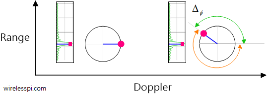
To avoid any unambiguity, this phase difference should be within $-\pi$ to $+\pi$, as illustrated in the figure below. If the phase at the next sweep has already crossed $\pi$ (shown by the orange arc), then this is known as aliasing and a ghost velocity will appear to the radar. This is similar to what happens when a ghost spectrum appear as a result of violating the sampling theorem.

Therefore, we can write
2\pi \frac{2vT_C}{\lambda} < \pi, \qquad \text{or}\qquad v_{max} = \frac{\lambda}{4T_C} \end{equation}
This result makes sense too. For measuring a higher velocity, phase angles should be taken more frequently. This results in a shorter chirp duration $T_C$.
Angular Resolution
This is an analogous case to velocity resolution. What is the minimum angle for which two targets appear as two separate peaks in the angle FFT output? This is illustrated in the figure below.

Using this Equation of Part 2,
\[
2\pi \frac{d\sin(\theta+\Delta\theta) -\sin\theta}{\lambda} \approx 2\pi \frac{d\cos \theta \Delta \theta}{\lambda}
\]
since the derivative of a sine is a cosine. Referring back to Eq (\ref{equation-fmcw-fft-resolution-discrete}), this turns out to be
\[
2\pi \frac{d\cos \theta \Delta \theta}{\lambda} > \frac{2\pi}{N}
\]
Thus the angular resolution is expressed as
\Delta\theta = \frac{\lambda}{Nd\cos\theta}
\end{equation}
Observe the following:
- Unlike velocity, the resolution itself depends on the angle $\theta$. This is due to the factor $\sin\theta$ and makes intuitive sense: two objects in front of the array can be better separated than those near the array axis.
- Similar to velocity where the resolution is inversely proportional to the frame length $T_f=NT_C$, the angular resolution is inversely proportional to the array length $Nd$.
Often this resolution is given for $\theta=0$ and the largest field of view, or $d=\lambda/2$.
\[
\Delta\theta = \frac{2}{N}
\]
Next, we describe the angular field of view for the array.
Angular Field of View (FOV)
This is an analogous case to maximum velocity. The maximum angle that can be extracted from the phase difference $\Delta_\phi$ in this Equation of Part 2 is
\[
\Delta_\phi = 2\pi \frac{d\sin\theta}{\lambda}
\]
To avoid any unambiguity, this phase difference should be within $-\pi$ to $+\pi$, as illustrated in the figure above. Therefore, we can write for two antennas,
2\pi \frac{d\sin\theta}{\lambda} < \pi, \qquad \text{or}\qquad \theta_{max} = \sin^{-1}\frac{\lambda}{2d} \end{equation}
This result makes sense too. For measuring a larger angle, phase values should be taken more frequently. This results in a shorter antenna spacing $d$. Notice the similarity with the maximum velocity calculation which is inversely proportional to the chirp duration $T_C$.
The largest field of view appears when $d=\lambda/2$ that produces $\theta_{max}$ equal to $\pm 90^\circ$, a spacing used in several implementations.
Summary
The equations in the red boxes above can be utilized as a starting point for an FMCW radar design procedure. When the product requirements such as distance and velocity resolutions as well as maximum range and velocity are given, the system parameters can be set by using those equations.
Calculate the parameters for a $77$ GHz FMCW radar with a range resolution of $10$ cm, velocity resolution of $1$ m/s, maximum distance of $100$ m and maximum velocity of $90$ km/hr.
- From Eq (\ref{equation-fmcw-range-resolution}), a range resolution of $10$ cm translates to a bandwidth of $B=1.5$ GHz.
- From Eq (\ref{equation-fmcw-maximum-velocity}), a maximum velocity of $90$ km/hr implies a chirp duration of $T_C \approx 40$ microseconds.
- From Eq (\ref{equation-fmcw-velocity-resolution}), a velocity resolution of $1$ km/hr means the frame duration should be $7$ milliseconds.
- Since the chirp rate $\mu=B/T_C$, it turns out to be $60$ MHz/microsecond. It is not always possible to design a device with such a chirp rate, so if a lower value of $\mu$ is chosen, the sweep time $T_C$ can be increased to achieve the same bandwidth $B$ and hence the range resolution. However, an increased $T_C$ would require settling for a lower maximum velocity.
- From Eq (\ref{equation-fmcw-maximum-distance}),the ADC sample rate $F_s$ determines the highest frequency $f_{b,max}$ that can be supported that in turn sets the maximum distance $d_{0,max}$.
Keep in mind that some of the requirements above can be in conflict with the hardware (e.g., filter bandwidth, ADC sample rate) and need to readjusted in tandem with the RF part.
This concludes our discussion on how an FMCW radar works. A review of limits for the design parameters is presented at the end.
Conclusion
The following table summarizes the design parameters in an FMCW radar.
| Resolution | Maximum | |
|---|---|---|
| Range | $\frac{c}{2B}$ | $\frac{cF_s}{2\mu}$ |
| Velocity | $\frac{\lambda}{2T_f}$ | $\frac{\lambda}{4T_C}$ |
| Angle | $\frac{\lambda}{Nd\cos\theta}$ | $\sin^{-1}\frac{\lambda}{2d}$ |
References
[1] M. Jankiraman, FMCW Radar Design, Artech House, 2018.
[2] S. Rao, Introduction to mmwave Sensing: FMCW Radars, Texas Instruments (TI) mmWave Training Series, 2017 – e2e.ti.com.


Hi Qasim
Thanks for excellent explanation of the FMCW RADARs. I was going thru the application note ‘SWRA553A–May 2017–Revised February 2020 Programming Chirp Parameters in TI Radar Devices’
On page 7, it mentions:
Max beat frequency 15 MHz
ADC sampling rate Msps 16.67
How can ADC sample 15MHz at 16.67 MHz without aliasing it ? AFAIK it must be twice of the max frequency ie. 2 x fbeat = 30 MHz.
The sampling theorem you know about (twice the maximum frequency) holds for real signals. For complex signals (see I/Q signals), there are already two real samples in each complex sample. Therefore, the sampling theorem for complex signals holds that the sampling frequency should be at least equal to the maximum frequency.
In your example, 16.67 MHz is slightly larger than 15 MHz since it gives transition bands of analog filters enough room to maneuver (a tight brick wall filter is not possible).
Thanks Qasim for quick response. Thanks again for this wonderful website and youtube tutorials.
There is a small error Eq 5 is Vres not Vmax. (However thanks for this very clear explanation)
Just fixed the typo. Thanks for letting me know.
Thank you so much Qasim, I am doing my SDP on FMCW Radar and your toturial is the best resource I found, books just through Eqs at you and I don’t have any background on radar to understand them. Thank you very much, I guess now I am ready to read books. I am so thankful for your great efforts!
Glad that it was helpful. All the best for your SDP. It will be a long road but applying your mind consistently to anything brings the desired fruits. It is the best feedback loop nature has invented.
Hi, from the example, i would like if you could elaborate the difference between the frame duration and chirp duration
A frame consists of $N$ consecutive chirps. In other words, the frame time $T_f$ is given by
\[
T_f = NT_C
\]
Hi Qasim,
It is amazing that you can explain such complex knowledge in an easy-to-understand way. Now I have an idea of how the radar detects/calculates the distance/speed of an object. This only covers one dimension, what I call depth to the observer. How can the radar determine the horizontal and vertical size/resolution from the observer’s perspective?
Sincerely,
David
Thanks for your kind words David. For that, you have to go one level higher towards receiving signals from multiple nodes; a single antenna can only do so much.
how do we ensure that we have a full cycle, meaning the beginning and end of the samples make a complete cycle, when getting the samples for FFT.
A radar is different than a communication receiver; it has full control of signal boundaries.
Hey Qasim, i wanted to what application you use to make such great math animations (waveforms,graphs,diagrams), i am asking because i have to use something similar for my project on FMCW radars for blind spot detection.
I use a combination of Python, Matlab and Visio (for block diagrams). Hope that helps.
thansk for the reply
Good day Qasim, i have one question, i currently am designing an FMCW radar using Adalm PLuto SDR for my FYP, one issue i have encountered is how to ensure The first sample of the Rx buffer must correspond to the first sample of the Tx chirp. Would you have any tips on how this can be done.
Most FMCW radar systems use a common clock to ensure precise timing between Tx and Rx operations. I think that the answer for what you are looking for is provided here.
Hi Qasim
I am currently modelling a fmcw radar system for only range estimation. I have during my modelling wondered if you know what benefits a I/Q mixer structure (2 mixers) has over just one ? I have been told that for one target alone the I/Q structure has computationally benefits as it find the distance estimate the phase by actan(I/Q) that can be used to find the distance compared to using FFT.
I would also like to ask you about the problem with FFT processing gain. I have gotten a pretty huge processing gain of 20 dB compared to my analog output when trying our differen peiods T. The SNR at the range I am measuring acording to friis should be drowned in noise but thanks to the processing gain I get from Bn =2/T it looks misrepresented in my plotting. Do you have any suggestion if this processing gain is a misrepresentation or not because there must be a limit on how long your chirp period can be or not ?
For your question 1, please see my article on I/Q signals which explains the benefits.
For your question 2, if the whole environment is completely stationary, and nothing changes, then you can have a long chirp and/or frame durations and enjoy huge processing gains. But any real environment is dynamic, even if the target does not move. This is why specifications of range and velocity resolutions and their maximum values are necessary.