Dec 04, 2020
There was a recent discussion on GNU Radio mailing list in regards to the simplest possible intuition behind I/Q signals. Why is I/Q sampling required?
Question: The original question from Kristoff went like this: “… when you mention `GNU Radio complex numbers’, you also have to mention I/Q signals, which is a topic that is very difficult to explain in 10 seconds to an audience who has never seen anything about I/Q sampling before.”
Comment: According to Jeff Long: “This is a great thing to try to figure out. If we can come up with an answer that gives someone a feel for why I/Q is used in SDR in 10 minutes, and does not include
- phasors,
- exponentials to a complex power,
- a derivation of any equation,
- the concept of orthogonality,
etc., … it will win a Nobel prize in education.”
This comment basically gives us a reasonably comprehensive list of traps to avoid to qualify for a good I/Q signals tutorial. Below, I attempt to explain this concept through one simple route, with an understanding that there are many other (better and more accurate) angles to view the same concept. Some remarks are in order here.
- There is no assumption of reader’s knowledge about introductory digital communications in this article. Therefore, I hope that SDR beginners will find these concepts easier to understand.
- Depending on your level of expertise, you can easily skip the sections you already know about.
- While the concept of I/Q signals applies to both a transmitter and a receiver, it is easier to understand it from a receiver perspective.
- I/Q signals are also called quadrature signals. We will shortly find out why.
Let us start with an introduction to an Electromagnetic (EM) wave.
An Electromagnetic Wave
Imagine a long straight wire with an AC source at its center shown in Figure 1. The source forces an acceleration and deceleration of charges in the forward and reverse directions. Since charges radiate whenever accelerated, the wire acts an antenna in which
- an electric field is produced due to the charge distribution, and
- a magnetic field is produced due to the varying current in the antenna.
The resulting Electromagnetic (EM) wave exhibits a sinusoidal form because the charges periodically travel back and forth to the ends of the wire. This wave propagates away from the source close to the speed of light in a direction perpendicular to both the electric and magnetic fields. A wireless signal is born.
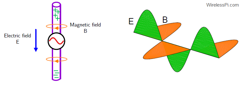
Figure 1: An electromagnetic wave is generated through acceleration of charged particles in a conductor in which the direction of propagation is perpendicular to both the electric and magnetic fields away from the source
A reverse process occurs on the receive side. The impinging EM wave influences the electrons in the antenna through its electric and magnetic fields. The acceleration and deceleration of these electrons under the influence of these fields creates a tiny electrical signal. This signal can be amplified and processed in any desirable manner.
More than 100 years ago, someone (there are some contestants to Marconi for this claim) figured out that a propagating electromagnetic wave can act as an information carrier to far away places without any physical connection, a revolutionary idea for the time. Then, some backed it up with actual demonstrations of wireless signal propagation, changing the world we live in forever. While the initial wireless transmission was based on analog communication like AM and FM, we skip that part and focus on digital modulation because it is both easy and relevant to understand.
For an unmodulated EM wave, the generated sinusoidal signal is given by
\begin{equation*}
s(t) = A\cdot \cos \left(2\pi Ft + \phi\right)
\end{equation*}
There are three different parameters that can be altered to transmit information.
- Amplitude $A$
- Frequency $F$
- Phase $\phi$
Such a cosine wave with amplitude $A=1$, frequency $F=1$ and phase $\phi=0$ is shown at the top left in Figure 2. Also indicated here are the respective phases through the duration of one full cycle. These angles come from the following relations.
\begin{align}
\cos 0^{\circ} \quad&= \quad 1 \nonumber\\
\cos 90^{\circ} \quad&=\quad 0 \nonumber\\
\cos 180^{\circ}\quad &=\quad -1 \label{equation-sinusoid}\\
\cos 270^{\circ} \quad&=\quad 0 \nonumber\\
\cos 360^{\circ}\quad &=\quad 1 \nonumber
\end{align}
where the angle $270^\circ$ is the same as $-90^\circ$. Also drawn in this figure are the cosine waves starting with a particular phase.
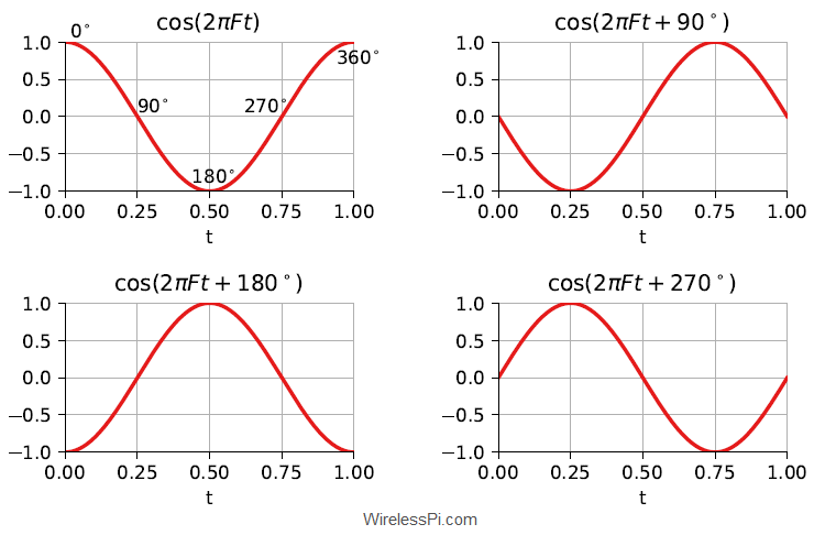
Figure 2: A cosine wave with different phases
- Notice that the phase of a sinusoidal wave just indicates the start time of that signal. While this is not necessary to understand this tutorial, ask me this question in the comments below if you are wondering about the reason and I will reply with an explanation.
- If the bottom right figure resembles a sine wave, this is because
\begin{equation}
\cos \left(2\pi Ft + 270^\circ\right) = \cos \left(2\pi Ft – 90^\circ\right) = \sin \left(2\pi Ft\right)
\end{equation}
To comprehend I/Q signals, is it helpful if we start with the three basic digital modulation schemes.
Frequency Shift Keying (FSK)
The simplest modulation scheme is Frequency Shift Keying (FSK) for which we discuss the binary case first. Also as far the general demodulation process is concerned, the reader should note that there are several different techniques for extracting the bits from the analog signal but I will only describe the simplest of algorithms in the spirit of this article.
FSK Modulation
In binary FSK, one frequency, say $F_0$, is transmitted for a logic 0 and another frequency, say $F_1$, is sent for a logic 1. An example BFSK waveform is drawn in Figure 3 for a bit stream given by
\begin{equation*}
1 ~~0~~1~~1~~0~~0
\end{equation*}
For each bit duration $m$ (I also call it a `signaling interval’ due to having a possibility of sending multiple bits on one waveform, as we will shortly find out), the modulated cosine waveform is written as
\begin{equation}\label{equation-fsk}
s(t) = A\cdot \cos \left(2\pi F_mt + \phi\right)
\end{equation}
where $F_m$ is either $F_0$ or $F_1$ depending on the data bit. We represent the phase here as a constant term $\phi$ but the actual waveform is slightly more complicated because the phase transitions at the boundaries of bit transitions are — in general — discontinuous. Ham radio operators usually call the signal representing the logic 1 as mark frequency and that representing logic 0 as space frequency.
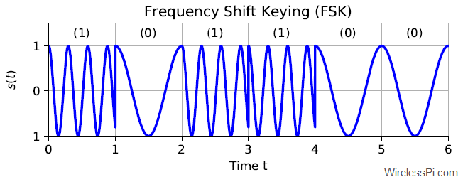
Figure 3: A Frequency Shift Keying (FSK) waveform with a lower frequency representing a 0 and a higher frequency representing a 1
Just as a reminder, one of the most interesting modulation schemes in digital communication, namely Minimum Shift Keying (MSK), is a version of FSK.
FSK Demodulation
In practice, an FSK signal can be demodulated through several methods such as quadrature demod, correlators or matched filtering, a Phase Locked Loop (PLL), bandpass filters, limiter discriminator, and so on. These methods can be broadly categorized as coherent versus non-coherent demodulation techniques. A coherent technique implies that a carrier waveform is available at the Rx that is phase and frequency aligned with the Tx waveform. On the other hand, a non-coherent technique ignores this phase difference between the devices and relies on alternative methods (e.g., envelop detection) for bit decisions. I will only consider a simple coherent technique here which is not only optimal in terms of bit error probability but you will also find it quite sensible when you think about it later.
An FSK waveform was described earlier as
\begin{equation*}
s(t) = A\cdot \cos \left(2\pi F_mt + \phi\right)
\end{equation*}
During each bit (or signaling) interval $m$, we receive a waveform with frequency $F_m$ that is a representation of the underlying bits. Consider a receiver synchronized with the transmitter in terms of carrier phase, carrier frequency and bit timing. To this end, we consider the following scenario.
- The frequency $F_0$, representing a 0, completes a single cycle in the bit interval $T_b$.
- The frequency $F_1$, representing a 1, is twice the frequency $F_0$.
The optimum implementation is a coherent demodulation scheme in which the Rx simply correlates two candidate carrier waves with the incoming waveform. By definition, correlation is a measure of similarity between two signals. In our everyday life too, we recognize something by correlating it with a stored image in our heads. As an example, in the The Hound of the Baskervilles, Sherlock Holmes accurately described Dr James Mortimer’s dog through correlating some observations with templates in his mind:
“… and the marks of his teeth are very plainly visible. The dog’s jaw, as shown in the space between these marks, is too broad in my opinion for a terrier and not broad enough for a mastiff. It may have been — yes, by Jove, it is a curly-haired spaniel.”
In the context of demodulating an FSK signal, correlation means that we multiply two candidate carrier waves in parallel at the Rx with the incoming waveform to check which one it resembles the most. One of these waves is $2\cos (2\pi F_0 t)$ while the other is $2\cos (2\pi F_1 t)$. This is shown in the block diagram of Figure 4. This whole process is similar to spotting an approaching dog and correlating its features with images of a spaniel and a mastiff in our minds.
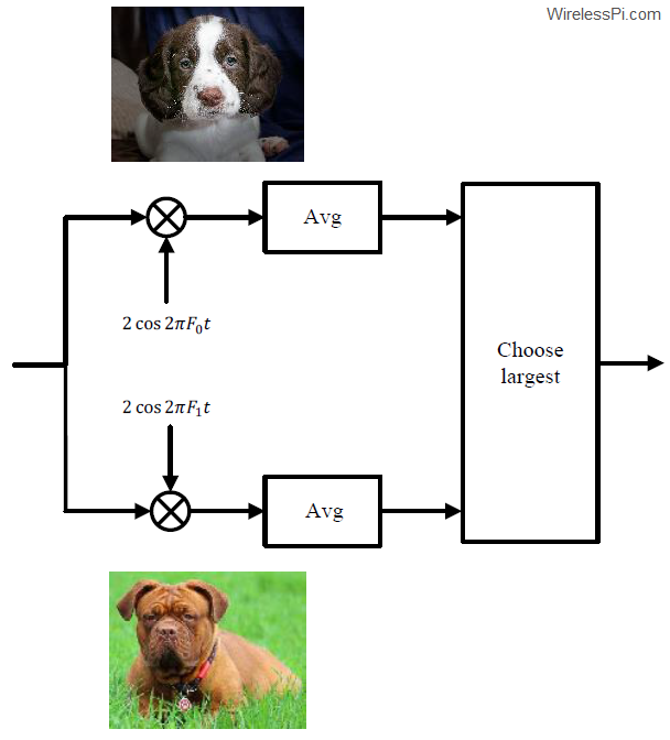
Figure 4: FSK demodulator block diagram
To quickly see why this procedure generates the correct output, consider the resulting waveforms drawn in Figure 5 corresponding to the block diagram of Figure 4. The multiplication operation by the same carrier generates two components, one at DC and the other at double the frequency. This is because
\begin{equation*}
\cos ^2 \theta = \frac{1}{2}+\frac{1}{2}\cos 2\theta
\end{equation*}
The averaging operation filters out high frequency terms in the output since averaging is a lowpass operation (e.g., averaging one full cycle of a sinusoid gives a zero output). Now let us examine what happens in the light of the two assumptions about $F_1$ and $T_b$ above.
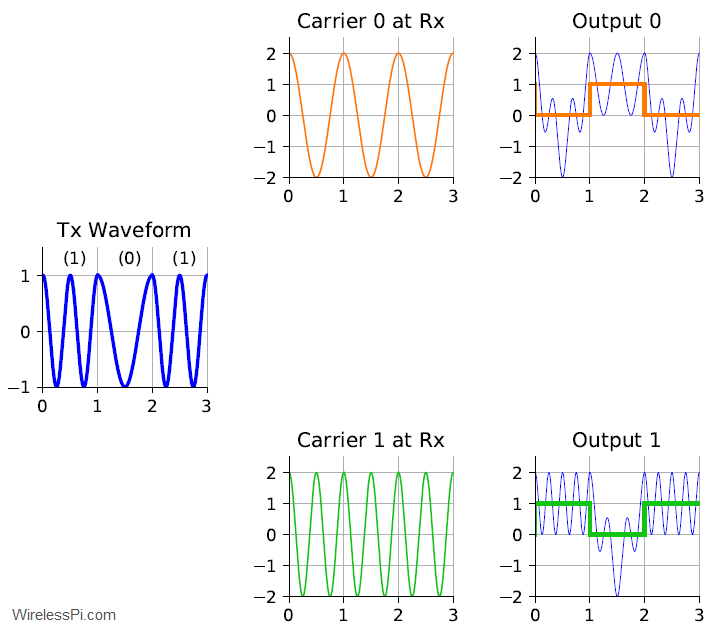
Figure 5: FSK demodulator waveforms
- In the upper arm, the product of cross-terms is a sum of two cosine waves, one at the difference frequency while the other at the sum frequency.
\[
\begin{aligned}
\underbrace{A\cdot \cos \left(2\pi F_1t\right)}_{\text{Incoming waveform}} \cdot \underbrace{2\cos\left( 2\pi F_0t \right)}_{\text{Generated at Rx}} &= \\
A\cdot \cos \left\{ 2\pi (F_1-F_0) t \right\}+&\underbrace{A\cdot \cos \left\{ 2\pi (F_1+F_0) t\right\}}_{\text{Filtered out}} \approx 0
\end{aligned}
\]where we have used the identity $2\cos\alpha \cos \beta$ $=$ $\cos (\alpha-\beta)$ $+$ $\cos(\alpha+\beta)$. After the averaging or filtering operation, a very small signal component remains (under ideal conditions) in the difference frequency term because sum of samples of this sinusoid in one period is zero. This zero value is shown at the top right of Figure 5 for the first bit.
- In the lower arm, we have
\begin{equation*}
\underbrace{A\cdot \cos \left(2\pi F_1t\right)}_{\text{Incoming waveform}} \cdot \underbrace{2 \cos\left( 2\pi F_1t \right)}_{\text{Generated at Rx}}= A+\underbrace{A\cdot \cos \left\{ 2\pi (2F_1) t\right\}}_{\text{Filtered out}} \approx A
\end{equation*}After the averaging or filtering operation, only the DC term $A$ remains (under ideal conditions). This is shown at the bottom right of Figure 5 for the first bit with $A=1$. Keep in mind that if the Tx and Rx frequencies were not aligned, the first term would also be time-varying with the difference frequency and if their phases were not aligned, a term $\cos (\phi-\phi’)$ would come with $A$ and potentially wipe it out (e.g., for a phase difference of $90^\circ$).
Thus for the first interval, the receiver decides in favour of bit 1. A similar process is repeated for the next arriving bits. Note that in the figure plotted here, I have chosen $F_1$ as an exact multiple of $F_0=1/T_b$ (i.e., $F_1=2F_0$) for showing a beautiful figure where both the cross-terms average out to zero. For each bit interval, the receiver carries out this product and averaging operation and chooses the frequency candidate with the largest output. For the chosen example, the receiver makes the following decisions.
\begin{align*}
\text{Bit interval 0} \quad \rightarrow \quad F_1 \quad \rightarrow \quad\text{Bit 1} \\
\text{Bit interval 1} \quad \rightarrow \quad F_0 \quad \rightarrow \quad \text{Bit 0} \\
\text{Bit interval 2} \quad \rightarrow \quad F_1 \quad \rightarrow \quad\text{Bit 1}
\end{align*}
Until now, we are doing just fine with one waveform that can be downcoverted and sampled. We have not encountered any need for I/Q signals yet (although I/Q sampling does make FSK demodulation much easier).
Amplitude Shift Keying (ASK)
In Amplitude Shift Keying (ASK), the signal amplitude $A$ (instead of frequency $F$) is used to indicate the value of a bit. Let us begin with a binary ASK system.
ASK Modulation
In a binary ASK system, we can transmit a sinusoidal waveform with one amplitude (e.g., $1$) for logic 0 and another amplitude (e.g., $2$) for logic 1, as shown in Figure 6. On a side note, On-Off Keying (OOK) is a special case of ASK in which the amplitude representing logic 0 is exactly $0$. In each signaling interval $m$, the resulting waveform is given by
\begin{equation}
s(t) = A_m\cdot \cos \left(2\pi Ft + \phi\right)
\end{equation}
where $A_m$ is either $1$ or $2$ according to the data bit.
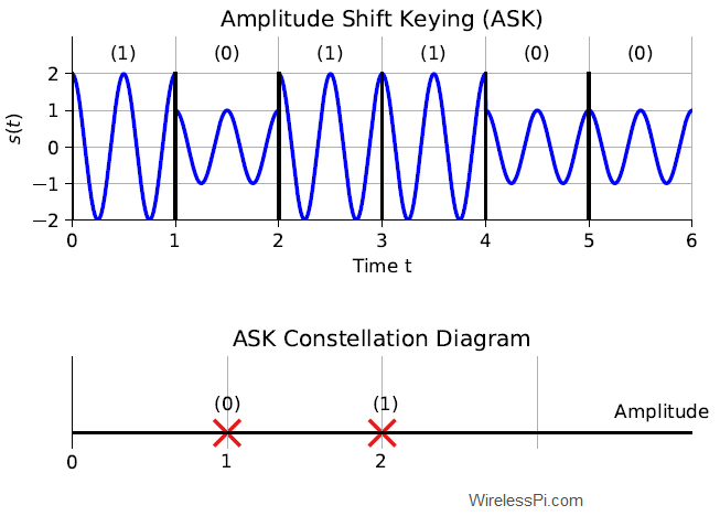
Figure 6: (Top) An Amplitude Shift Keying (ASK) waveform with a lower amplitude representing a 0 and a higher amplitude representing a 1. (Bottom) An ASK constellation diagram
You would have noticed in Figure 6 that the choice of the two amplitudes is poor as we focus on their positive values only. Such a representation is commonly known as unipolar ASK. The alternative is bipolar ASK where the amplitudes are instead chosen as $+1$ and $-1$. In most cases, bipolar ASK is preferred over unipolar ASK due to power and bit error rate performance. Nevertheless, a negative sign indicates a change in phase of $180^\circ$ and our main purpose is to clearly distinguish this waveform from Phase Shift Keying (PSK) which comes next.
Here, I introduce you to something known as a constellation diagram. It is a representation of a digital modulation scheme independent of the underlying carrier waveform. For example, a constellation diagram for a binary ASK scheme showing the two information carrying amplitudes, $1$ and $2$, is drawn in Figure 6. You can relate this to the actual waveform in the following manner. For sending a logic 0, the carrier wave is multiplied with a value of $1$ and for a logic 1, it is multiplied with a value of $2$.
These points shine like stars in a night sky. The purpose of a constellation diagram is to bypass all the less relevant signals and focus solely on the parameter that carries the actual digital information.
ASK Demodulation
An ASK waveform was described earlier as
\begin{equation*}
s(t) = A_m\cdot \cos \left(2\pi Ft + \phi\right)
\end{equation*}
During each bit (or signaling) interval $m$, we receive a waveform with amplitude $A_m$ that is a representation of the underlying bits. Consider a receiver synchronized with the transmitter in terms of carrier phase, carrier frequency and bit timing. For the demodulation of ASK signals, we can follow a similar procedure as FSK and correlate (i.e., multiply and average) the incoming waveform with two carrier waves of different amplitudes generated at the Rx. Consider a received signal with an amplitude $2$ (representing bit 1) in the first interval.
- In the upper arm, we can have
\begin{equation*}
A_1\cdot \cos \left(2\pi Ft +\phi\right) \cdot 2A_0\cdot \cos\left( 2\pi Ft +\phi\right)
\end{equation*} - In the lower arm, we can have
\begin{equation*}
A_1\cdot \cos \left(2\pi Ft +\phi\right) \cdot 2A_1\cdot \cos\left( 2\pi Ft +\phi\right)
\end{equation*}
However, the carrier wave in both cases is exactly the same, so why produce it twice and multiply it twice? A better option is to generate a single carrier with frequency $F$ and simply check the output amplitudes after a filtering or averaging operation. It can be easily seen from above that such an output would be $A_m$ depending on the data bit and the corresponding amplitude.
\begin{equation*}
\underbrace{A_m\cdot \cos \left(2\pi Ft +\phi\right)}_{\text{Incoming waveform}} \cdot \underbrace{2 \cos\left( 2\pi Ft +\phi\right)}_{\text{Generated at Rx}}= A_m+\underbrace{A\cdot \cos \left\{ 2\pi (2F) t + 2\phi\right\}}_{\text{Filtered out}} \approx A_m
\end{equation*}
Observe that the frequency $F$ and phase $\phi$ must be the same for such a cancellation to happen for the first term. In practice, this is accomplished through carrier phase synchronization and frequency synchronization algorithms while the optimal instants for decision samples are found through timing synchronization procedure. This is drawn in the right column of Figure 7 where the output amplitudes are 2, 1 and 2 corresponding to the three bits are 1, 0 and 1, respectively. The double frequency terms are also visible in the background that are filtered out.
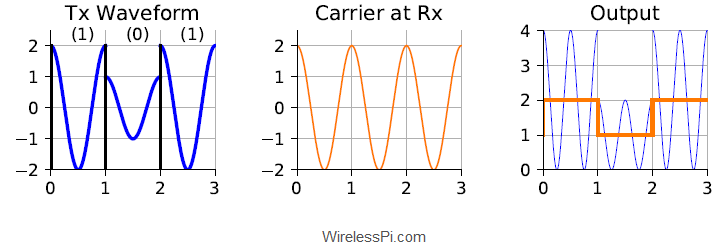
Figure 7: ASK demodulator waveforms
Again observe that we are doing just fine without any I/Q signals. Demodulating the signal from a single carrier waveform seems enough.
Granularity on the Axis
We have learned above that a Tx and Rx agree upon the modulation choice which forms the basis for the algorithms required for the detection of bits. When a digitally modulated waveform is received, the Rx extracts the information carrying parameter and maps those levels at the Rx constellation onto the designated bits. As opposed to the simple constellation diagrams for binary modulations shown above, more than two points are needed in a real constellation as follows.
Higher-Order Modulations
Digital electronics are constrained to work on only two levels by electronic switches which in the simplest case are either on or off. Actual digital communication systems require quite complicated signal processing workload both at the Tx and Rx ends that can be performed only by a device more intelligent than an electronic switch, such as an Application Specific Integrated Circuit (ASIC), Field Programmable Gate Array (FPGA), Digital Signal Processor (DSP) or a General Purpose Processor (GPP).
Hence if a Rx can differentiate between two signal levels to detect which bit was sent, it can also differentiate between more than two signal levels. Being able to do so can result in sending more data during the same amount of time. In this system, multiple bits (say, $2$) can be collected during every unit of time, converted into their decimal equivalents and one level out of possible options (e.g., $2^2=4$) can be accordingly selected for transmission.
In the case of 4-FSK for instance, this implies that four different carrier frequencies can be utilized where each of them represents a set of two bits.
\begin{align*}
F_0 \quad &\rightarrow \quad 00 \\
F_1 \quad &\rightarrow \quad 01 \\
F_2 \quad &\rightarrow \quad 10 \\
F_3 \quad &\rightarrow \quad 11 \\
\end{align*}
For example, the Figure 8 shows a new waveform for an FSK modulation with four different frequencies each representing two bits. The bit sequence is as follows.
\begin{equation*}
1~~1~~0~~0~~1~~0~~0~~1
\end{equation*}
From this bit sequence, two bits are collected at each instant as 11, 00, 10 and 01 and carrier waves with the corresponding frequencies $F_3$, $F_0$, $F_2$ and $F_1$, respectively, are sent over the air. These bit assignments are arbitrary (e.g., bits 00 can be sent through frequency $F_2$) as long as the Tx and Rx agree on the same convention.
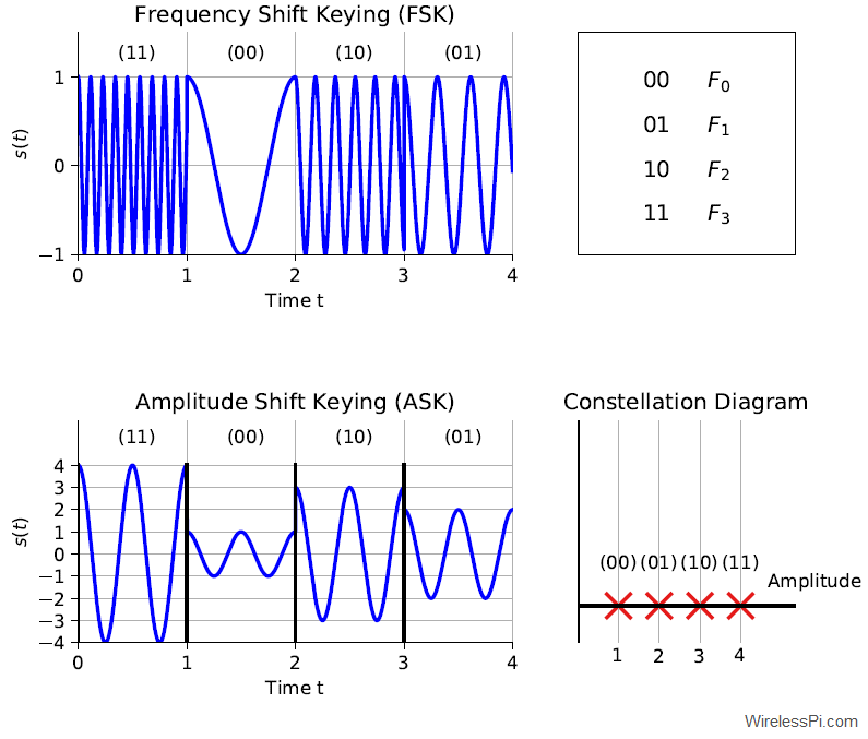
Figure 8: (Top) An FSK signal with 4 levels. (Bottom) An ASK signal with 4 levels along with its constellation diagram
In Figure 8, carefully map each set of two bits to their respective frequency to grasp how the waveform is generated. For example, according to the assignment on the right, the first two bits 11 are assigned to the frequency $F_3$. Therefore, the frequency $F_3$ (which happens to be the highest) is sent during the first signaling interval. On the same note, $F_0$ is transmitted during the second interval due to the bits being 00, and so on.
A similar phenomenon occurs for ASK modulation systems. More number of bits can be sent through inclusion of higher or lower amplitudes according to the target number of bits. A 4-ASK constellation diagram is shown in Figure 8 where each amplitude represents a set of $2$ bits. The difference here as compared to FSK is that these levels are assigned to the amplitude of a carrier wave with a single frequency. Some comments are in order here.
- The most relevant observation is that these additional amplitudes lie on the same axis of the constellation diagram.
- What happens when more than $2$ bits (e.g., $3$) need to be packed in each transmission interval? We can simply increase the number of levels to $2^3=8$. Note that in all these cases, either higher or lower amplitudes are added to this group but the growth stays on the same axis of the constellation diagram.
- As far as the demodulation is concerned, it follows the same principles described before.
In conclusion, a higher granularity of more than two modulation levels are required for higher-rate schemes.
Mismatches between Parameters
Even for a binary modulation scenario, a finer resolution on the constellation diagram is needed. This is because no two Tx and Rx devices are the same and there is always a mismatch between their parameters. In the FSK case for instance, the frequency of the local oscillator at the Rx is not exactly the same as the carrier of the incoming signal and there is always some difference between the manufacturer’s nominal specification and the real frequency of that device. This is known as a carrier frequency offset. Moreover, this offset keeps varying (slightly) with temperature, pressure, age and other factors. Consequently, instead of only two frequencies, we need a continuum of levels on that frequency axis (you can read about how a Direct Digital Synthesizer (DDS) can be used for signal generation at any frequency).
In an ASK system too, the absolute Rx amplitude is affected by several factors such as channel attenuation and path loss. Again, we need a continuum of amplitudes for Rx constellation mapping. This is where phase as a parameter is different from frequency and amplitude, as we explain now.
Phase Shift Keying (PSK)
In Phase Shift Keying (PSK), the data is transmitted by changing the phase of a constant frequency carrier wave at each signaling interval.
PSK Modulation
In the binary case here, two different phases are employed to represent the bit values. For example, logic 0 and logic 1 are sent with phases $0 ^\circ$ and $180^\circ$ of the carrier wave, respectively. This waveform is drawn below for the same bit sequence as before. Look specifically at the bit boundaries to notice the phase transitions. The waveform for each interval $m$ is
\begin{equation}
s(t) = A\cdot \cos \left(2\pi Ft + \phi_m\right)
\end{equation}
where $\phi_m$ is $0^\circ$ or $180^\circ$ depending on the data bit. If you have a confusion regarding these phases, refer to the cosine figure at the start of this article where we connected the phase relations of Eq (\ref{equation-sinusoid}) to the waveform values.
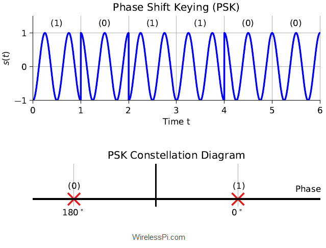
Figure 9: (Top) A Phase Shift Keying (PSK) waveform with phase 0 representing a 0 and phase pi representing a 1. (Bottom) A PSK constellation diagram
The constellation diagram for a binary PSK scheme is also shown in the same figure where the carrier phase is chosen as either $0^\circ$ or $180^\circ$ according to the incoming bit. Otherwise, the waveform frequency and amplitude stay the same in both cases.
PSK Demodulation
Something really interesting happens when it comes to demodulating a PSK signal. Consider a receiver synchronized with the transmitter in terms of carrier phase, carrier frequency and bit timing. For the demodulation of PSK signals, we can
- either follow a similar procedure as FSK and correlate the incoming waveform with two carrier waves of different phases generated at the Rx,
- or follow a similar procedure as ASK and correlate (i.e., multiply and average) the received waveform with a single carrier to observe its phase.
Since the amplitude and frequency stay the same for all phases, it makes sense (and can be proved to be optimal) to adopt the second route above. If the Tx and Rx frequencies are exactly the same and their phase difference is also equal to zero except the modulation phase $\phi_m$, we can write
\begin{equation*}
\underbrace{A\cdot \cos \left(2\pi Ft +\phi_m\right)}_{\text{Incoming waveform}} \cdot \underbrace{2 \cos\left( 2\pi Ft\right)}_{\text{Generated at Rx}}= A\cdot \cos \phi_m+\underbrace{A\cdot \cos \left\{ 2\pi (2F) t + \phi_m\right\}}_{\text{Filtered out}} \approx \cos \phi_m
\end{equation*}
for $A=1$ and where we have used the identity $2\cos\alpha \cos \beta$ $=$ $\cos (\alpha-\beta)$ $+$ $\cos(\alpha+\beta)$. After the averaging or filtering operation, only the DC term $\cos \phi_m$ remains (under ideal conditions). Looking at this term $\cos \phi_m$, here is the interesting observation I hinted at earlier.
\begin{equation*}
\cos 0^\circ = 1 \qquad \text{and} \qquad \cos 180^\circ = -1,
\end{equation*}
such a demodulation process has transformed the phases into amplitudes!
This is drawn in Figure 10 where the three bits are 1, 0 and 1 and the corresponding output amplitudes are -1, +1 and -1.
\begin{align*}
\text{Bit interval 0} \quad \rightarrow \quad -1 \quad \rightarrow \quad 180^\circ \quad \rightarrow \quad \text{Bit 1} \\
\text{Bit interval 1} \qquad \rightarrow \quad +1 \quad \rightarrow \quad 0^\circ \quad \rightarrow \quad \text{Bit 0} \\
\text{Bit interval 2} \quad \rightarrow \quad -1 \quad \rightarrow \quad 180^\circ \quad \rightarrow \quad \text{Bit 1}
\end{align*}
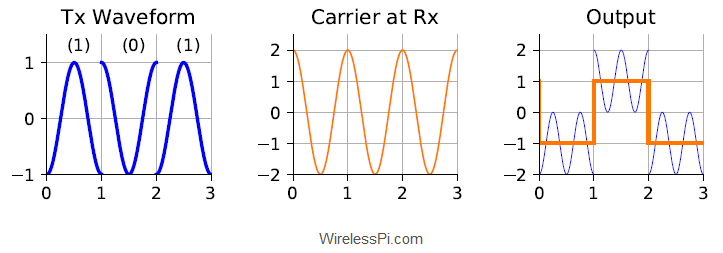
Figure 10: PSK demodulator waveforms
A question that arises is the following. Instead of converting the phase into amplitude, is it possible to build an algorithm that directly detects the phase for each bit interval? This is related to I/Q sampling as we find out next.
From Geometrical Angle to Signal Phase
Observe from the ASK constellation diagram that all the amplitudes still extend on the same axis. On the other hand, for a PSK system, one axis is not enough because an actual angle is formed by two lines, not one. This is shown in Figure 11. In other words, an ASK modulation scheme has a 1-dimensional constellation diagram while a PSK system requires a 2-dimensional constellation diagram. And that has made all the difference, as we shortly see.
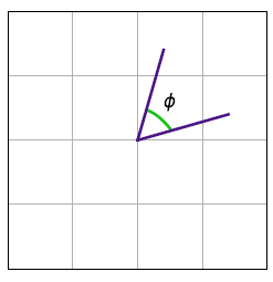
Figure 11: An angle is formed by two lines, not one
Let us explore this concept with respect to both higher-order modulations and phase offsets.
4-PSK Example
Previously we described a 2-PSK system where a phase of $0^\circ$ represents bit 0 while a phase of $180^\circ$ represents bit 1. Now for a 4-PSK modulation, we can send a set of two bits during each signaling interval as follows.
\begin{equation*}
\begin{aligned}
0^{\circ} \quad &\rightarrow \quad 00 \\
90^{\circ} \quad &\rightarrow \quad 01 \\
180^{\circ} \quad &\rightarrow \quad 10 \\
270^{\circ} \quad &\rightarrow \quad 11 \\
\end{aligned}
\end{equation*}
These phases are shown in the constellation diagram of Figure 12 along with their bit assignments. As noted earlier, these bit assignments are arbitrary and can be altered easily as long as the Tx and Rx keep the same table. Let us explore how the modulated waveform is generated for the same bitstream.
\begin{equation*}
1~~1~~0~~1~~1~~0~~0~~0
\end{equation*}
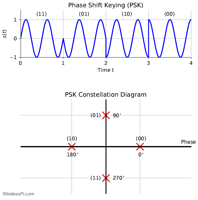
Figure 12: A PSK signal with 4 levels along with its constellation diagram
First, refer to the cosine figure at the start of this article that connects the angle relations in Eq (\ref{equation-sinusoid}) to the phases of the sinusoidal waveform. Now the first two bits in the stream are 11 which map to the last phase, i.e., $270^\circ$. This implies that the cosine wave should start at the second zero crossing. This can also be seen from
\begin{equation*}
\cos (\theta + 270^\circ) = \cos (\theta – 90^\circ) = \sin \theta
\end{equation*}
and hence the waveform in the first signaling interval has a sine shape. The next set of bits is 01 which implies that the cosine wave has a phase of $90^\circ$ in the second interval. You can follow the same logic for the rest of the signal representing the bits 10 and 00.
8-PSK with a Phase Offset
Even for a binary PSK system, a finer phase resolution is needed at the Rx due to a phase offset between the Tx and Rx. Some factors that contribute towards this phase offset are mismatched time references between Tx and Rx local oscillators, overall channel impulse response (including all the analog and digital filtering) and the propagation delay between the two devices.
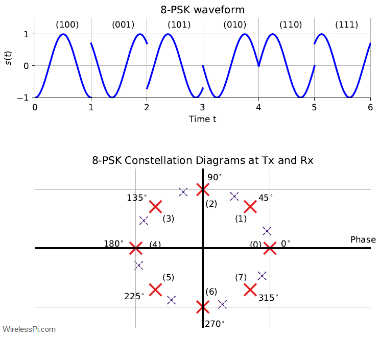
As an example, an 8-PSK waveform is drawn in Figure 13 for a bit sequence
\begin{equation*}
\underbrace{1~~0~~0}_{4}~~\underbrace{0~~0~~1}_{1}~~\underbrace{1~~0~~1}_{5}~~\underbrace{0~~1~~0}_{2}~~\underbrace{1~~1~~0}_{6}~~\underbrace{1~~1~~1}_{7}
\end{equation*}
Notice the phase transitions at the signaling boundaries where the waveform phase is altered to represent each new set of 3 bits entering the modulator. The waveform is not joined at these boundaries to highlight these fine phase changes. With the experience of previous PSK figures, I hope that the reader can map the waveform boundary phases to the Rx constellation diagram. For example, the first 3 bits represent are 100 which represent a decimal value of 4. On the constellation diagram at the bottom, 4 corresponds to an angle of $180^\circ$ (starting from $0$). Therefore, the first signaling interval shows a cosine wave with a $180^\circ$ phase.
In Figure 13, the Tx constellation can be located at an angle spacing of $45^\circ$ on the unit circle that dictates the waveform phases drawn above. However, the Rx constellation is drawn with a phase offset of $17^\circ$ as dotted lines. This is done in order to demonstrate that the actual phase can lie anywhere in this 2-D plane (although this phase offset is not included in the actual top waveform).

Figure 13: (Top) An 8-PSK waveform. (Bottom) Two constellation diagrams: one at the Tx shown by thick red lines and the other at the Rx for a phase offset of 17 degrees shown by dotted purple lines
Demodulation with Cosine
Let us apply the same demodulation algorithm used for binary PSK before. This is what happens for each signaling interval.
- The incoming signal is multiplied with a single carrier wave.
- The output is averaged or filtered.
- The resulting amplitudes are marked on the Rx constellation diagram (e.g., $+1$ and $-1$ in binary PSK).
With this algorithm, we said that if the Tx and Rx frequencies are exactly the same and their phase difference is also equal to zero except the modulation phase $\phi_m$, we can write
\begin{equation*}
\underbrace{A\cdot \cos \left(2\pi Ft +\phi_m\right)}_{\text{Incoming waveform}} \cdot \underbrace{2 \cos\left( 2\pi Ft\right)}_{\text{Generated at Rx}}= A \cdot \cos \phi_m+\underbrace{A\cdot \cos \left\{ 2\pi (2F) t + \phi_m\right\}}_{\text{Filtered out}} \approx \cos \phi_m
\end{equation*}
for $A=1$ and where we have used the identity $2\cos\alpha \cos \beta$ $=$ $\cos (\alpha-\beta)$ $+$ $\cos(\alpha+\beta)$. After the averaging or filtering operation, only the DC term $\cos \phi_m$ remains (under ideal conditions). Now we apply such a demodulation procedure to an 8-PSK waveform of Figure 13 for which the results are drawn in Figure 14.
- In the first signaling interval, the output amplitude is $-1$ which refers to a phase of $180^\circ$. An arrow shows the output amplitude $-1$ in the third subplot going to $-1$ in the Rx constellation diagram of the last subplot. Mapping to the Tx constellation diagram of Figure 13 (shown by thick red lines) tell us that the corresponding baud is 4 which translates to a 3-bit sequence of 100. Hence, our first 3 detected bits are 100. So far so good.
- Let us skip the next interval to avoid having an arrow crossing over other segments. In the time interval between $2$ to $3$, the output is
\begin{equation*}
-0.707 = -\frac{1}{\sqrt{2}} = \cos 135^\circ
\end{equation*}Can we map it back to a geometrical angle? Not exactly because cosine of $225^\circ$ is also exactly the same! We do not have a unique angle and corresponding bit map in this case. This also becomes clear by looking at the Tx constellation diagram of Figure 13 where cosine of both $135^\circ $ and $225^\circ$ cast a shadow at $-0.707$ on the real line.
- This situation becomes even more tricky in the fourth and fifth signaling intervals where the demodulator output in the third subplot is zero in both instances. This is shown by an arrow mapping the $0$ amplitude in both cases to $0$ in the Rx constellation diagram. Looking at the top of Figure 14 reveals that cosine wave actually started from different phases (i.e., $+90^\circ$ for (2) and $-90^\circ$ for (6), respectively). However, its shadow on the real line should be at $0$ for both points.
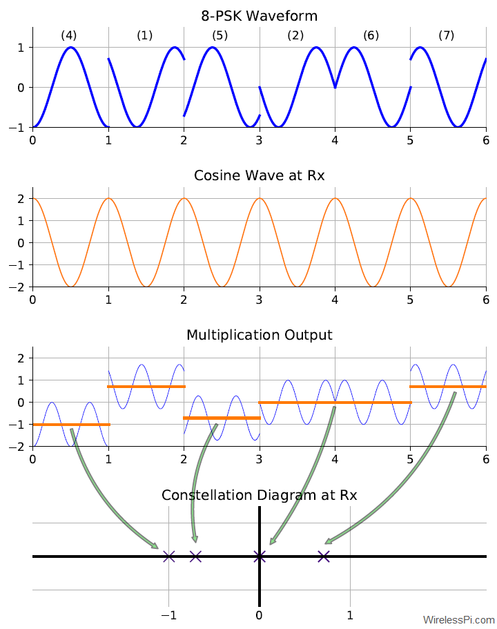
Figure 14: Demodulation process of an 8-PSK waveform with a cosine wave
A Naive Algorithm
It might seem that the problem is with this demodulation procedure which converts the phase into amplitude for decision making. A naive algorithm here could work as follows.
Take many samples of the cosine wave in each signaling interval and record the starting value. Then, compute the slope of the wave at this point to estimate the actual underlying phase. While there are dozens of implementation issues with this approach but suffice it to say that this will require an insanely large number of extremely low-noise samples for each such duration. I mentioned this algorithm here because I remember someone making this suggestion somewhere.
I/Q Sampling
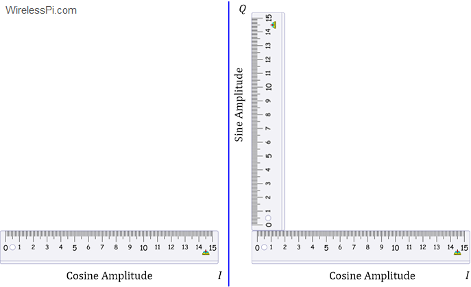
This brings us to the solution. Recall from Figure 11 that an angle is made up of two lines, not one.
This means that we need two points to represent an angle, not one! One such point gives the amplitude on the horizontal axis and the other point gives the amplitude on the vertical axis. When we attempted to tie the concept of a geometrical angle with a waveform phase, we completely forgot during demodulation that only one amplitude is being extracted here — the one representing the horizontal axis.
Question: How should we extract the amplitude on the vertical axis?
Answer: We need another waveform at the Rx!
Question: If the horizontal axis links angle $0^\circ$ on a 2-D plane to a cosine wave with the starting phase $0^\circ$, then the vertical axis at an angle $90^\circ$ on a 2-D plane should be linked to which waveform?
Answer: Another cosine wave with the starting phase of $90^\circ$.
Question: What is a cosine wave with a starting phase of $90^\circ$?
Answer: Use the identity $\cos(\alpha+\beta)$ = $\cos\alpha \cos \beta$ – $\sin\alpha \sin \beta$.
\begin{equation*}
\cos \left (2\pi F t + 90^\circ\right) = \cos 2\pi F t \cdot \underbrace{\cos 90^\circ}_{0} – \sin 2\pi Ft\cdot \underbrace{\sin 90^\circ}_{1} = – \sin 2\pi Ft
\end{equation*}
This second cosine wave comes out to be a negative sine wave!
In conclusion, in parallel with the cosine wave starting with a phase of $0^\circ$, we need another cosine wave at the Rx starting with a phase of $90^\circ$, which is a negative sine wave. All this means that a cosine wave measures the x-axis projection of the phase like a ruler and hence cannot measure the actual angle. We need two rulers to estimate the full angle, where $I$ length is provided by the cosine and $Q$ length is provided by the negative sine, see the figure below.
\[
\measuredangle (\cdot) = \tan^{-1}\frac{Q}{I}
\]
Keep in mind that we will see the more technical definition of an angle shortly. In summary, what we are doing here is that instead of measuring the angle (e.g., through a protractor), we are measuring the two amplitudes (represented by lengths below) and estimating the angle through their ratio! This is because amplitudes are much easier to work with as compared to angles.
Let us run the same demodulation algorithm for the same bit sequence as in Figure 14 but multiply the arriving signal with a negative sine wave (instead of a cosine signal). The results of these operations are plotted in Figure 15.
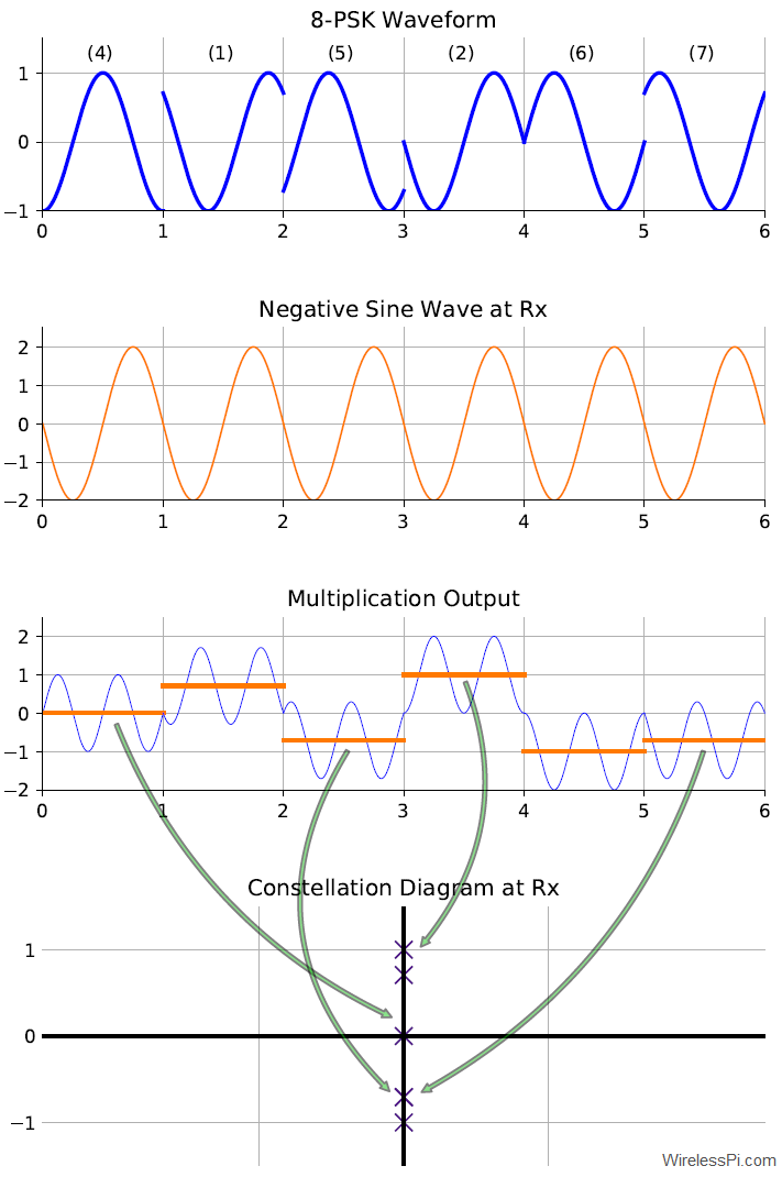
Figure 15: Demodulation process of an 8-PSK waveform with a negative sine wave
If the Tx and Rx frequencies are exactly the same and their phase difference is also equal to zero except the modulation phase $\phi_m$, we can write
\begin{equation*}
\underbrace{A\cdot \cos \left(2\pi Ft +\phi_m\right)}_{\text{Incoming waveform}} \cdot \underbrace{\left\{-2 \sin\left( 2\pi Ft\right)\right\}}_{\text{Generated at Rx}}= A \cdot \sin \phi_m-\underbrace{A\cdot\sin \left\{ 2\pi (2F) t + \phi_m\right\}}_{\text{Filtered out}} \approx \sin \phi_m
\end{equation*}
for $A=1$ and where we have used the identity $-2\cos\alpha \sin \beta$ $=$ $\sin (\alpha-\beta)$ $-$ $\sin(\alpha+\beta)$. After the averaging or filtering operation, only the DC term $\sin \phi_m$ remains (under ideal conditions). Consequently, the output amplitudes then map to the correct point in a 2-D plane as
\[
(x, y) = (\cos \phi_m, \sin \phi_m)
\]
We connect this result to the output waveform in Figure 15 now. For this purpose, we repeat the bit sequence examined earlier for convenience.
\begin{equation*}
\underbrace{1~~0~~0}_{4}~~\underbrace{0~~0~~1}_{1}~~\underbrace{1~~0~~1}_{5}~~\underbrace{0~~1~~0}_{2}~~\underbrace{1~~1~~0}_{6}~~\underbrace{1~~1~~1}_{7}
\end{equation*}
- In the first signaling interval, the output amplitude is $0$. Recalling that the result of cosine multiplication in Figure 14 was $-1$, the point on the 2-D plane is given by
\[
(x, y) = (-1, 0)
\]Mapping to the Tx constellation diagram of Figure 13 (shown by thick red lines) gives us the first 3 bits as 100.
- In the time interval between $2$ to $3$, the output is $-0.707$. It was also $-0.707$ for cosine multiplication due to which the point on 2-D plane is
\begin{equation*}
(x, y) = (-0.707, -0.707)
\end{equation*}
While initially we had a confusion between the candidate being $135^\circ$ or $225^\circ$, we can simply locate this point in the middle of the 3rd quadrant and hence find the correct angle as $225^\circ$. Therefore, the data bits are completely resolved corresponding to number (5) as 101. - The fourth and fifth signaling intervals, while zero for cosine demodulation, are now $+1$ and $-1$, respectively. From the constellation diagram of Figure 13, the points on 2-D plane are $(0, +1)$ and $(0, -1)$ which map to data points (2) and (6), respectively. Therefore, the bits in the fourth signaling interval are 010 while those in the fifth signal interval are 110. This can be checked by the top waveform in Figure 15.
Let us now learn the rationale behind the terms $I$ and $Q$.
Rationale Behind the Terms $I$ and $Q$
Each phase, like each angle, needs a reference. For the angles, this reference is provided by the horizontal line connecting point $(0,0)$ to point $(1,0)$.
- For the phases, we choose a cosine wave with phase $0^\circ$ as the reference (as is clear from the previous sections). Therefore, an amplitude modulated cosine wave is known as the “In-Phase” component, from which the notation $I$ is extracted. Sometimes, the $I$ term refers only to the amplitude riding over this cosine wave and represented by the value on the x-axis.
- On the same note, an amplitude modulated sine wave, which has a phase difference of $90^\circ$ with the reference cosine wave, is known as the “quadrature” component, from which the notation $Q$ is extracted. Sometimes, $Q$ refers only to the amplitude riding over this sine wave and represented by the value on the y-axis. In general, quadrature refers to the position of a planet when it is $90^\circ$ from the sun as viewed from the earth.
Phase Computation
With points mapped on a 2-D plane, one question is the following. How is phase computed from those $I$ and $Q$ components? For this purpose, a function known as four-quadrant inverse tangent is employed. This is different than the regular inverse tangent function because it takes into account all four quadrants. For an amplitude of $A_I$ on $I$-axis and $A_Q$ on $Q$-axis, the angle $\measuredangle$ is defined in terms of $\tan^{-1} (A_Q/A_I)$ below. If you find it complicated, just remember that it is a way of computing the correct quadrant from the signs of $I$ and $Q$ amplitudes.
\begin{equation*}
\measuredangle (\cdot) =
\begin{cases}
\tan^{-1} \frac{A_Q}{A_I} & A_I > 0 \\
\tan^{-1} \frac{A_Q}{A_I} + \pi & A_I < 0 \mbox{ and } A_Q \ge 0\\
\tan^{-1} \frac{A_Q}{A_I} – \pi & A_I < 0 \mbox{ and } A_Q < 0\\ +\pi/2 & A_I = 0 \mbox{ and } A_Q > 0\\
-\pi/2 & A_I = 0 \mbox{ and } A_Q < 0
%\mbox{indeterminate } & A_I = 0 \mbox{ and } A_Q = 0.
\end{cases}
\end{equation*}
Computing such a function is not easy in real-time at a high rate but many algorithms have sprung up for this purpose after the advent of Software Defined Radios (SDR).
What If You Have Only 5 Minutes?
What will you say if you have only 5 minutes to explain someone the concept of I/Q signals? One suggestion is to explain the implementation of Quadrature Amplitude Modulation (QAM).
We have learned that PSK modulation chooses discrete phases on the same circle. Moreover, I/Q refers to points on a 2-D plane and hence I/Q data involves both amplitude and phase of the carrier. So why do modulation points necessarily have to be on the same circle? They don’t have to. Since discrete amplitudes can be chosen in ASK modulation, we can combine one amplitude and one phase at each signaling interval. Such a strategy gives rise to the most widely used digital modulation technique known as Quadrature Amplitude Modulation (QAM). Let us discuss this concept through a QAM modulator and demodulator that form the backbone of your WiFi, cellular and other high rate communication systems.
Modulator
For each signaling interval $m$, start with a waveform modulated in both amplitude and phase as
\begin{equation}\label{equation-qam}
s(t) = A_m\cdot \cos \left(2\pi Ft + \phi_m\right)
\end{equation}
Using the identity $\cos (\alpha+\beta)$ $=$ $\cos\alpha \cos \beta$ $-$ $\sin \alpha \sin \beta$, open this up as
\begin{align}
s(t) &= A_m\cdot \cos (2\pi Ft)\cdot \cos \phi_m – A_m \cdot \sin 2\pi Ft \cdot \sin \phi_m \nonumber\\
&= \underbrace{(A_m\cos \phi_m)}_{\text{I part}}\cdot \cos (2\pi Ft) – \underbrace{(A_m \sin \phi_m)}_{\text{Q part}} \cdot \sin 2\pi Ft \label{equation-qam-iq}
\end{align}
Here, the amplitude $A_m\cos \phi_m$ is the projection of the modulation point on $x$ or $I$ axis, while the amplitude $A_m\sin \phi_m$ is the projection of the modulation point on $y$ or $Q$ axis. This is plotted in Figure 16. These amplitudes are then modulated on two quadrature carriers, namely $\cos (2\pi Ft)$ and $-\sin (2\pi Ft)$ and summed together to be sent over the air. Notice that both of these carriers are zero-phase sinusoids, as compared to the single amplitude+phase modulated sinusoid in Eq (\ref{equation-qam})!! And again, it’s much easier to work with amplitudes.
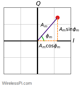
Figure 16: I/Q plane and modulation parameters
A modulator can generate a QAM waveform either through direct modulation as in Eq (\ref{equation-qam}), or through $I$ and $Q$ waveforms as in Eq (\ref{equation-qam-iq}). The latter route is simpler as it only involves amplitude modulation of two quadrature waveforms with no need to alter the phase. A block diagram for implementing a QAM modulator is shown in Figure 17. The filtering shown here is a specialized operation known as pulse shaping.
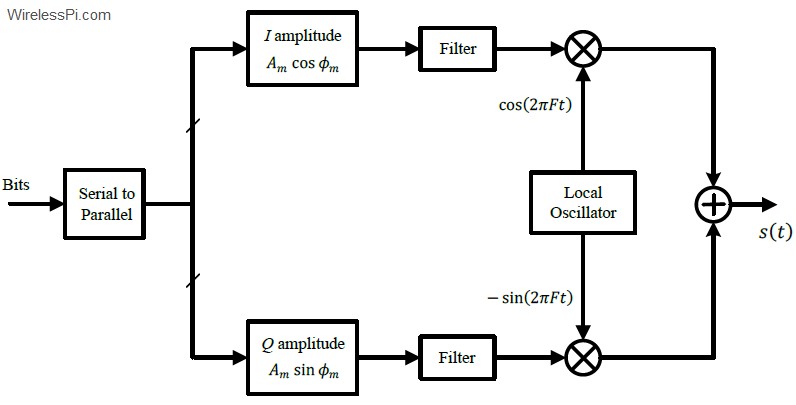
Figure 17: A block diagram for a QAM modulator
Demodulator
At the Rx side, multiply the incoming signal with the two quadrature waveforms, namely $\cos (2\pi Ft)$ and $-\sin 2\pi Ft)$, in parallel. A block diagram for a QAM demodulator is drawn in Figure 18. The filtering shown here is a specialized operation known as matched filtering. The idea is similar to a correlator we saw in FSK demdoulator but matched to the pulse shape at Tx side. An Analog-to-Digital (A/D) conversion is casually shown here, the exact place of which depends on the receiver architecture employed (e.g., a superheterodyne receiver). Also, the whole point of software defined radios was to perform this conversion as close to the antenna as possible. After A/D conversion, the samples are mapped to the Rx constellation shown as four stars. Each decision is made in favour of a star closest to the received data point. You can learn more about QAM here.
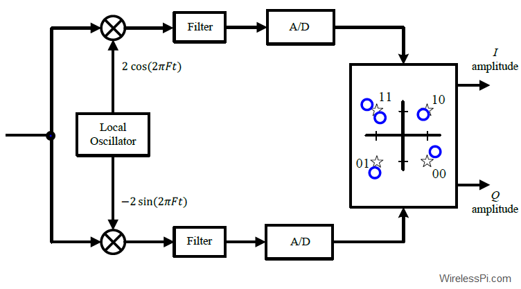
Figure 18: A block diagram for a QAM demodulator
With frequency, phase and timing synchronization in place, the process is as follows.
- In the $I$ arm, we have
\begin{equation*}
\begin{aligned}
s(t)\cdot 2 \cos\left( 2\pi Ft\right) &= \underbrace{A_m \cdot \cos \left(2\pi Ft +\phi_m\right)}_{\text{Incoming waveform}} \cdot \underbrace{2 \cos\left( 2\pi Ft\right)}_{\text{Generated at Rx}} \\ &= A_m \cdot \cos \phi_m+\underbrace{A_m\cdot \cos \left\{ 2\pi (2F) t + \phi_m\right\}}_{\text{Filtered out}} \approx A_m \cos \phi_m
\end{aligned}
\end{equation*} - In the $Q$ arm, we have
\begin{equation*}
\begin{aligned}
s(t)\cdot \left\{-2 \sin\left( 2\pi Ft\right)\right\} &= \underbrace{A_m \cdot \cos \left(2\pi Ft +\phi_m\right)}_{\text{Incoming waveform}} \cdot \underbrace{\left\{-2 \sin\left( 2\pi Ft\right)\right\}}_{\text{Generated at Rx}} \\ &= A_m \cdot \sin \phi_m-\underbrace{A_m\cdot \sin \left\{ 2\pi (2F) t + \phi_m\right\}}_{\text{Filtered out}} \approx A_m \sin \phi_m
\end{aligned}
\end{equation*}
This is drawn in Figure 19 for the following example amplitudes and phases.
\begin{equation*}
A_m = \{1, 2, 1\} \qquad \qquad \phi_m = \{45^\circ, 135^\circ, 270^\circ\}
\end{equation*}
The reader can easily trace the arrows to see that for the second signaling interval, for instance, $2\cdot \cos 135^\circ$ $=$ $-1.41$ and $2\cdot \sin 135^\circ$ $=$ $+1.41$ are correctly being mapped. The same holds true for the last interval where $1\cdot \cos 270^\circ$ $=$ $0$ and $1\cdot \sin 270^\circ$ $=$ $-1$.
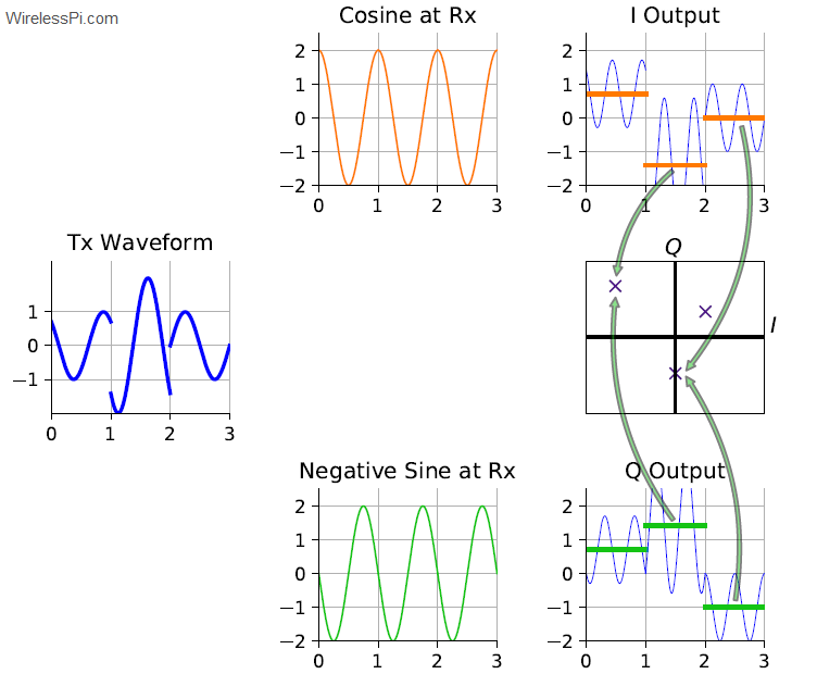
Figure 19: I/Q demodulation process and projections on I and Q axes
We did not go into details here but I/Q signals are very helpful for implementation of any modulation scheme. Also keep in mind that I and Q components of a signal without the carrier wave can be treated as the real and imaginary parts of a complex number.
Concluding Remarks
This concludes our discussion on I/Q signals. You can learn this concept from an even more fundamental viewpoint in the article Two birds with one tone: I/Q signals and Fourier Transform.
Interestingly, only experienced engineers in the past could design such communication systems due to the specialized electronics knowledge required for implementing mathematical relations through electronic circuits. The revolution brought by SDRs is that the same relations can be implemented through any programming language much more conveniently. This has opened the door for hobbyists and amateurs to build close to professional-grade communication systems in just two steps.
- You can create the Tx/Rx code in a graphical programming environment like GNU Radio which are called flowgraphs. Example flowgraphs for QAM and PSK modulation schemes can be found here.
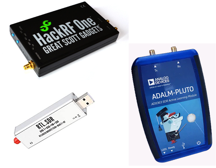
- Connect an SDR hardware like RTL-SDR, HackRF or ADALM Pluto to your computer (or use a free SDR) and include the relevant device driver (available in the form of a graphical block) into your code above.


Amazing. Great work. I was wondering what happen if we use any encoding and decoding techniques? How does this work ? Let’s say if you use CDMA with spreading factor 8, how does one can co-relate?
Thanks. In the case of CDMA, the receiver has to correlate the incoming signal with the intended sequence. The sequence with the user’s code will have the highest correlation while other sequences output a low value that will appear as additional noise in the user’s signal after despreading.
Great explanation. Thank you. Keep up the good work.
Glad you liked it.
Really liked the article. Very informative. Keep on posting this kind of articles.
Glad you liked it.
Hi! This was very good. I’m squeaky new to the IQ signal world and I’m building my knowledge. I had two questions that might sound silly.
So the first is when you were solving the equations you mentioned “average or filtering” what exactly did you mean by this because I didn’t follow the math.
The second question is, I thought I/Q components needed a carrier wave of some sort, but in one of your closing statements you mentioned that without a carrier wave these were real and imaginary parts of a complex number, what were you trying to get at exactly? I guess I see how they would be a real and imaginary part but I don’t know how it relates to waves.
Thank you!
Thanks for your kind words. And no question is ever silly.
1. Averaging or filtering – If you look at those FSK equations, there is a difference frequency $F_1-F_0$ and a sum frequency $F_1+F_0$. Naturally, the sum frequency is the higher one. Filtering implies removing some part of the spectrum. A lowpass filter filters out the higher frequencies. An averaging operation is a rectangular signal in time domain and has a sinc shape in frequency domain that is essentially a lowpass filter. You can read more about filters here and about averaging operation here.
2. Complex numbers and waves – Complex numbers were invented (not discovered) around 500 years ago. The idea is to have a balancing representation for ‘impossible powers’ of x. This idea carried itself into waves (in studies of engineering and science) because although wave amplitudes and frequencies are real and can fit in one dimension, we need two dimensions to represent its phase (remember phase is related to angle?). This is why complex numbers and then complex signals were a perfect fit for wave representation. You can read more about it in a real-imaginative guide to complex numbers.
Thank you for your beautiful explanation
Could u explain this
“Notice that the phase of a sinusoidal wave just indicates the start time of that signal. While this is not necessary to understand this tutorial, ask me this question in the comments below if you are wondering about the reason and I will reply with an explanation”
Consider the sinusoidal wave
\[
x(t) = \cos (2\pi ft)
\]
If it is delayed by an amount $t_0$, then it incurs a phase $\theta$ as
\[
\cos (2\pi f (t-t_0)) = \cos (2\pi ft + \theta)
\]
We can say that the phase $\theta$ is given by
\[
\theta = -2\pi ft_0
\]
that is directly proportional to the time shift $t_0$. You can see further details in my article on the effect of time shift in frequency domain.
Qasim,
You provided the best explanation I never found anywhere else regarding IQ data. A non-scientist can read and understand the whole concept. Just to wanted to say thank you!
Eva, your compliment is much appreciated.
Thanks for this great article. I finally understand the purpose of having both I and Q.
I am left wondering, however, why PSK is preferred if it’s essentially doubling the work (not to mention adding the inverse tangent)?
Why not just add as many logic levels as you need on the 1 dimensional FSK or ASK, and save processing time?
Hi Joe,
I’m sorry I somehow missed your question. PSK is spectrally more efficient than FSK and ASK. For the same amount of energy spent, it yields a higher bits/second/Hz, see the spectral efficiency idea here.
Reading a RTL-SDR doc, it’s said that RTL2832U supports tuners at IF (Intermediate Frequency, 36.125MHz), low-IF (4.57MHz), or Zero-IF output using a 28.8MHz crystal. Based on the above proof, how can a zero-IF be used to get IQ and still downconverts incoming signals with higher carrier frequency? Or, how zero-IF works? A mathematical explanation may be much appreciated. Thanks for your clarity to demistify concepts for “low IQ” people like me. Thanks.
I also saw that you have an online book. I will get it at some point and even advertise.
Intermediate Frequency (IF) is different than carrier frequency. In other receiver architectures, the modulated signal is brought down to an intermediate frequency (mentioned in your examples) before final downconversion to baseband. In zero-IF architecture, the modulated signal is downconverted directly to the baseband. Writing mathematical details here isn’t possible due to space constraints; Chapter 10 of my Wireless Communications book contains these details.
I want to purchase your book but cannot find it on amazon, could you please advise on how to get your book.
You can purchase the Wireless Comms eBook at the link below (the whole package includes an SDR course with GNU Radio exercises plus a Project, and a 5G PHY eBook).
Wireless Comms eBook + SDR Course + 5G PHY eBook
If you are interested in the hard copy of Wireless Comms book only, then you can order it at the link below.
Wireless Comms on Amazon
Hi Qasim, my doubts
1) How is the complex number and complex signals are related in 2D plane. How can i interpret the (YI, YR) 2D plane (u mentioned in real imaginative article) with (I,Q) signals 2D plane(current article)?
2) QAM uses 2 amplitude axis to determine phase. Is there any modulation scheme uses 3 amplitude axis (3D plane) to determine constellation in space? Likewise can we go with multiple dimensions?
Interesting questions.
1) All signals are made up of waves. A wave has different phases that can be decomposed into in-phase (cosine) and quadrature (sine) components. Therefore, the value of a single wave at a particular phase is exactly that of a zero-phase cosine and a sine with amplitudes determined from the amplitude and phase of the original.
2) It’s the same question as asking if complex numbers have 2 dimensions, which numbers have 3 dimensions. From a communications perspective, we utilize higher dimensions of orthogonality between cosines, sines, etc. through Orthogonal Frequency Division Multiplexing (OFDM). Keep in mind that I and Q are still there in OFDM from a carrier frequency perspective but several higher dimensions, e.g., $N=64$ or more, from baseband perspective.
Thanks for the excellent explanation! In figure 17 could you please clarify if the output s(t) is a digitally modulated signal ? Would a DAC be the next stage in this figure before frequency up conversion and amplification ?
Very good question. I drew this figure for illustrative purpose only. In practice, the waveform will be generated in digital domain and the placement of DAC depends on the exact receiver architecture. For a general modem, please see the article on Quadrature Amplitude Modulation (QAM).
Hi Qasim,
Thank you for this great article. I have a question though – in Fig. 17, shouldn’t the filter be placed AFTER the mixer (instead of before) in order to remove the unwanted beat frequencies?
Thanks for your kind words Rakesh. There are no beat frequencies here. This filter in Fig. 17 actually does the following.
You can read how this is done in the articles on pulse shaping and upsampling a signal.
Thanks for this great article. I finally understand the purpose of having both I and Q.
I am left wondering, however, why PSK is preferred if it’s essentially doubling the work (not to mention adding the inverse tangent)?
Why not just add as many logic levels as you need on the 1 dimensional FSK or ASK, and save processing time?
Excellent question. For the same average energy, the points are packed in a better manner in 2-D constellations than in 1-D constellations. This results in better immunity against the noise which translates in an improved symbol error rate. See the article on computing error rates in different modulations.
“There is no assumption of reader’s knowledge about introductory digital communications in this article. Therefore, I hope that SDR beginners will find these concepts easier to understand.”
I’ve been in the field for over 15 years, and you already lost me at the first equation in the first section. This is definitely NOT beginner friendly.
Thanks for your feedback Dan. Do you mean the equation below?
\begin{equation*}
s(t) = A\cdot \cos \left(2\pi Ft + \phi\right)
\end{equation*}
I assumed knowledge of cosine and sines since these are taught in high school. Maybe you will find the next tutorial on I/Q signals I wrote easer to understand?
Hello Qasim, that’s some of the great explanation of the concept.
I have a quick doubt: The IQ concepts have been beautifully explained looking with the perspective of receivers, but we do have this concept on the transmitter side, isn’t it?
Thank you so much for your effort again!
I mean, is it only for the QAM case we would need or can it be made useful for any other modulation as well?
Thank you. Yes, it is useful for transmitter side as well as receiver side, wherever 2D signal processing is involved. It is true for all modulations including Frequency Shift Keying (FSK). See the tutorial that covers even more fundamental ideas of I/Q signals and Fourier Transform here.