Having built a simple digital communication system, it is necessary to know how to measure its performance. As the names say, Symbol Error Rate (SER) and Bit Error Rate (BER) are the probabilities of receiving a symbol and bit in error, respectively. SER and BER can be approximated through simulating a complete digital communication system involving a large number of bits and comparing the ratio of symbols or bits received in error to the total number of bits. Hence,
\begin{equation}\label{eqCommSystemSER}
\text{SER} = \frac{\text{No. of symbols in error}}{\text{Total no. of transmitted symbols}}
\end{equation}
and
\begin{equation}\label{eqCommSystemBER}
\text{BER} = \frac{\text{No. of bits in error}}{\text{Total no. of transmitted bits}}
\end{equation}
Till now, the only imperfection between Tx and Rx entities we have covered is AWGN. It then makes sense that more distortions should corrupt the signal further and result in more errors. Hence, SER or BER plotted against some measure of signal-to-noise ratio (SNR) is the benchmark against which the performance of a system can be measured. Another useful parameter that combines the effects of all impairments into a single value is Error Vector Magnitude (EVM).
Next, we discuss how we choose a specific measure of SNR against which SER and BER should be plotted.
Figure of Merit: $E_b/N_0$
The SNR in a digital communication system is defined as a ratio of signal power in a symbol $P_M$ to noise power $P_w$ as
\begin{equation}\label{eqCommSystemSNR}
SNR = \frac{P_M}{P_w}
\end{equation}
where the signal power $P_M$l is modulation average symbol energy per unit symbol time
\begin{equation}\label{eqCommSystemPowerEnergy}
P_M = \frac{E_M}{T_M}
\end{equation}
For PAM and QAM modulation schemes, average $E_M$ was defined in their respective articles, see Pulse Amplitude Modulation (PAM) and Quadrature Amplitude Modulation (QAM). Moreover, how to determine the noise power $P_w$ was detailed in the article on AWGN.
When specified in dB units and using a factor of 10 for power conversions, it is
\begin{align}
SNR_{\text{dB}} &= P_{M,\text{dB}} – P_{w,\text{dB}} \nonumber \\
&= 10 \log_{10} P_M – 10\log_{10} P_w \label{eqCommSystemSNRdB}
\end{align}
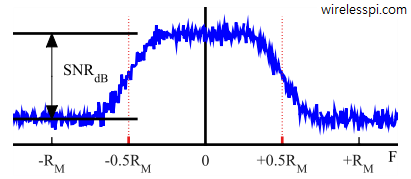
A visual measure of finding $\mathrm{SNR_{dB}}$ is shown in Figure below.
Using Eq \eqref{eqCommSystemPowerEnergy} and Eq \eqref{eqCommSystemNoisePower1}, notice that the SNR can also be written as
\begin{align*}
P_M \cdot \frac{1}{P_w} &= \frac{E_M}{T_M} \cdot \frac{1}{N_0 B} \\
&= E_M R_M \cdot \frac{1}{N_0B}
\end{align*}
The above equation can be rearranged as
\begin{equation*}
\frac{E_M}{N_0} = \frac{P_M}{P_w} \cdot \frac{B}{R_M}
\end{equation*}
Recall that there are $\log_2 M$ bits in one symbol,
\begin{equation}\label{eqCommSystemEMEb}
E_b = \frac{1}{\log_2M} \cdot E_M
\end{equation}
where $E_b$ is energy per bit. Similarly, the bit rate is
\begin{equation}\label{eqCommSystemRMRb}
R_b = \log_2 M \cdot R_M
\end{equation}
Plugging the values for $E_b$ and $R_b$,
\begin{equation}\label{eqCommSystemEbNo}
\frac{E_b}{N_0} = \frac{P_M}{P_w} \cdot \frac{B}{R_b} = \text{SNR} \cdot \frac{B}{R_b}
\end{equation}
So we can say that $E_b/N_0$ is equal to SNR scaled by ratio of bandwidth to bit rate.
Now the question is: why is $E_b/N_0$ a natural figure of merit in digital communication systems instead of SNR.
- Intuitively, the ratio of signal power $P_M$ to noise power $P_w$ in the system (i.e., SNR) should be a good criterion for measuring performance of different communication systems. And indeed it is true for analog communication systems where the signal continuity transcends the need to partition the signal into some units of time. On the other hand, a symbol is the basic building block of a digital communication system and signal energy within each symbol turns out to be a more useful parameter.
- As we saw in the article on packing more bits in one symbol, many bits ($\log_2M$ to be precise) can be packed into every symbol for an $M$-symbol modulation. Consequently, within every $T_M$ seconds, either 1 bit is travelling through the air (BPSK), or 2 bits (QPSK, 4-PAM), or 4 bits (16-QAM, 16-PSK), and so on. As shown in Eq \eqref{eqCommSystemEbNo}, using $E_b/N_0$ instead of SNR automatically incorporates this bits per symbol factor through $R_b$.
- Again from Eq \eqref{eqCommSystemEbNo}, bandwidth is also taken into account. A system using less bandwidth than the other will have this factor reflected in its $E_b/N_0$ values.
In summary, $E_b/N_0$ is a normalized SNR measure, which proves really useful when comparing the SER/BER performance of digital modulation schemes with different bits per symbol and bandwidths.
The ratio $E_b/N_0$ is dimensionless as
\begin{equation*}
\frac{E_b}{N_0} = \frac{\text{Joules}}{\text{Watts/Hz}} = \frac{\text{Watts} \cdot \text{seconds}}{\text{Watts} \cdot \text{seconds}}
\end{equation*}
It is frequently expressed in decibels as $10\log_{10} E_b/N_0$.
Scaling Factors
In most of the figures in this text, you would have noticed a very clear labeling on the x-axis. On the y-axis though, the emphasis has been on the shape rather than the exact values. Now when the SER/BER measurements are to be taken, scaling factors on y-axis become equally important.
Constellation
Starting with the symbol constellations, we scale the values such that the average energy per symbol is 1. This can be achieved by dividing the constellation values by the square root of average symbol energy (sum of squares of the constellation points). For example, for a PAM modulation with $A=1$, $E_M$ was shown to be equal to
\begin{equation*}
E_{M-\text{PAM}} = \frac{M^2-1}{3}
\end{equation*}
which yields
\begin{align*}
E_{2-\text{PAM}} &= 1 \\
E_{4-\text{PAM}} &= 5 \\
E_{8-\text{PAM}} &= 21 \\
\vdots
\end{align*}
When the constellation points $\pm 1$, $\pm 3$, $\pm 5$, $\cdots$, are divided by respective $\sqrt{E_M}$, various $M$-PAM constellations become normalized to have average symbol energy equal to $1$, as illustrated in Figure below.
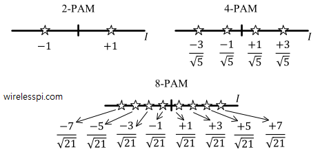
As a verification, consider from Figure above,
\begin{align*}
E_{2-\text{PAM,norm}} &= \frac{1}{2}\left(1^2 + 1^2\right) = 1 \\
E_{4-\text{PAM,norm}} &= \frac{1}{4}\cdot \frac{1}{5}\left(-3^2 + -1^2 + 1^2 + 3^2 \right) = \frac{1}{20}\cdot 20 = 1 \\
E_{8-\text{PAM,norm}} &= 1
\end{align*}
where the subscript `norm’ stands for normalized.
On a similar note, the scaling factor for QAM with $A=1$ was shown as
\begin{equation*}
E_{M-\text{QAM}} = \frac{2}{3} \left(M-1\right)
\end{equation*}
which yields
\begin{align*}
E_{4-\text{QAM}} &= 2 \\
E_{16-\text{QAM}} &= 10 \\
E_{64-\text{QAM}} &= 42 \\
\vdots
\end{align*}
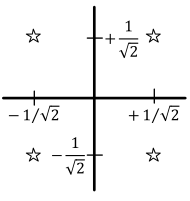
For example, when scaled with square-root of this normalization factor, a normalized $4$-QAM constellation is shown in Figure below. Here, using Pythagoras theorem and realizing that all $4$ symbols have equal energies,
\begin{equation*}
E_{4-\text{QAM,norm}} = \frac{1}{4}\cdot 4\cdot \left(\frac{1}{2} + \frac{1}{2} \right) = 1
\end{equation*}
Observe that the constellation points come closer to each other for higher-order modulation and normalized average symbol energy. This emphasizes the fact that higher bit rate $R_b$, or more bits per symbol, does not come for free. The tradeoffs involved are
- Power needs to be increased for a fixed bandwidth, because more energy within the same symbol time is needed for maintaining a similar distance between constellation points, or
- Bandwidth needs to be expanded to accommodate a higher symbol rate for fixed power, because same energy then becomes available to spend during a shorter amount of time, or
- An increased error rate needs to accepted for fixed power and bandwidth.
Tx Pulse
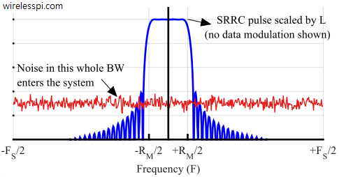
To understand the scaling factor for Tx pulse shape, also known as Tx filter, consider the block diagram of a PAM modulator or a QAM modulator. The next step after converting bits to symbols is upsampling the symbol train before it is filtered by a square-root Nyquist filter. This square-root Nyquist filter performs two operations:
- It lowpass filters the spectral replicas arising as a result of increasing the sample rate, see the post on sample rate conversion for details.
- It shapes the symbol sequence so that it is bandlimited in the frequency domain according to given specifications.
We also discussed in sample rate conversion that to maintain the same peak time domain amplitude in the upsampled signal as before, the filter should be designed with a gain equal to the upsampling factor, $L$ in this case. The three available choices, time domain amplitudes and energies were presented there. When we choose this option, the symbol energy gets scaled by $L$ as well as derived in that post. Therefore, denoting energy/symbol in the upsampled and filtered case with $E’_M$,
\begin{equation}\label{eqCommSystemScalingEnergy}
E_M’ = L \cdot E_{M\text{,norm}} = L
\end{equation}
Remember from the post on pulse shaping filter that the peak value in a Square-Root Raised Cosine filter is $1 – \alpha + 4\alpha/\pi$. In an actual implementation of the system, the pulse coefficients should be scaled by this value as well so that the peak value becomes unity and the precision with which the coefficients are represented in a fixed-point arithmetic processor can be maintained. However, here the purpose is only to simulate the BER due to which we ignore this factor.
Noise Power
In the article on AWGN, the noise power $P_w$ within a bandwidth $B$ was derived as
\begin{equation}\label{eqCommSystemNoisePower1}
P_w = N_0B
\end{equation}
For a discrete signal with sampling rate $F_S$, it is understood that the bandwidth has already been constrained by an analog filter within the range $\pm 0.5F_S$ to avoid aliasing. Plugging $B=0.5F_S$ in the above equation, the noise power in a sampled bandlimited system is given as
\begin{equation*}
P_w = N_0\cdot \frac{F_S}{2}
\end{equation*}
A digital modulation signal is sampled at rate $F_S = L \cdot R_M$ where $L$ is samples/symbol. Bit rate $R_b$ can change with different modulation schemes and sample rate $F_S$ can be increased or decreased during the processing chain. On the other hand, the symbol rate $R_M$ is a standard parameter which is directly proportional to the signal bandwidth as shown in the modulation bandwidths, and hence it remains constant throughout the system implementation. For this reason, $R_M$ in most simulation systems is chosen to be equal to $1$ and the other parameters can be scaled accordingly. Then,
\begin{equation}
P_w = N_0\cdot \frac{L}{2} \label{eqCommSystemNoisePower2}
\end{equation}
Finally, the relationship between noise power $P_w$ and $E_b/N_0$ can be written as
\begin{equation*}
P_w = \frac{E_b}{E_b/N_0} \cdot \frac{L}{2}
\end{equation*}
which can be modified using $\log_2 M$ bits per symbol,
P_w = \frac{E_M}{\log_2 M \cdot E_b/N_0} \cdot \frac{L}{2}
\end{equation}
where $E_M$ is the symbol energy. In case normalized energy is used for symbol constellations, it can be replaced with $1$.
Notice that noise power increases by a factor of $L$ due to oversampling the signal. On the other hand, the signal energy increases by a factor of $L$ due to scaling shown in Eq \eqref{eqCommSystemScalingEnergy}. The overall result is that both factors cancel out in the numerator and denominator of SNR expression in Eq \eqref{eqCommSystemSNR}. This is illustrated in Figure below.
Rx Pulse
Both the signal and noise enter the system before filtered by the Rx pulse. Therefore, any scaling has no effect on the SNR and it only changes the time domain amplitudes. Since the Raised Cosine pulse is a convolution of Tx and Rx Square-Root Raised Cosine pulses defined above, it has a peak amplitude of $1$ and hence maps the symbols exactly on the constellation.
Finally, remember that the group delay defined in pulse shaping filter is now given by the contribution from both Tx and Rx square-root Nyquist filters. For that reason, we remove $LG/2+LG/2=LG$ samples at the start and $LG$ samples at the end of the received sequence.
BER Plots
Now we are at a stage where we can plot the symbol and bit error rates of all three modulation schemes discussed above, namely PAM, QAM and PSK. To avoid any confusion, we leave SER plots and just concentrate on BER plots. SER plots are an obvious byproduct of the simulation setup discussed above.
The BER plots for 2, 4 and 8-PAM modulation are shown in Figure below.

Note that for a fixed $E_b/N_0$, the BER increases with $M$ because the same symbol energy has to be divided among $\log_2M$ bits. Similarly, for a fixed BER, more energy is required as $M$ increases to maintain similar distances among constellation points. As an example, for a target BER of $10^{-4}$,
- $E_b/N_0$ needed by $2$-PAM is $8.4$ dB,
- $E_b/N_0$ needed by $4$-PAM is $12.2$ dB,
- $E_b/N_0$ needed by $8$-PAM is $16.5$ dB,
A gray code is a method of assigning bits to symbols in a manner that adjacent symbols differ in only one bit. For example, symbols in a $4$-PAM constellation can be assigned bits 00, 01, 11 and 10 (as opposed to 00,01,10 and 11) such that all symbols have neighbours with only one bit difference. Since Gaussian noise has a higher probability around the mean value, the most likely symbol errors end up in adjacent symbols. As a result, these most likely symbol errors produce one erroneous bit and remaining $M-1$ correct bits. Hence, the relation between BER and SER can be defined as
\begin{equation*}
\text{BER} = \frac {1}{\log_2 M} \text{SER}
\end{equation*}
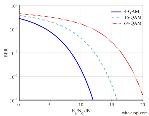
Moving on to QAM, the BER plots for $4$, $16$ and $64$-QAM modulation are shown in Figure beow. Similar conclusions hold for BER vs $E_b/N_0$ as in the case of PAM.
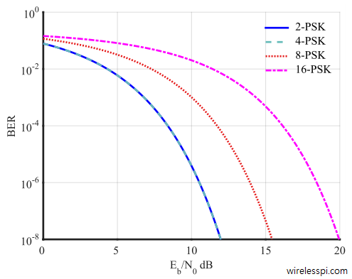
Finally, the BER plots for 2, 4 ,8 and 16-PSK modulation are shown in Figure below. Notice that the plots for BPSK and QPSK overlap with each other because QPSK can be regarded as a pair of orthogonal BPSK systems. We will have more to say about this point in the next section.
Spectral Efficiency
In BER vs $E_b/N_0$ plots above, we noticed that for a target BER of $10^{-4}$, $E_b/N_0$ required by $2$-PAM, $4$-PAM and $8$-PAM are $8.4$ dB, $12.2$ dB and $16.5$ dB, respectively. Does this mean that $8$-PAM is $8$ dB worse than $2$-PAM modulation scheme? The answer is no, because the bandwidth has not been taken into consideration in this comparison. For the same symbol rate (which means same bandwidth), $8$-PAM transmits $3$ bits of information as compared to just $1$ bit of information by $2$-PAM.
For that reason, bandwidth must also be considered to get a complete picture of how different modulations compare to one another. Thus, spectral efficiency is defined as the ratio of bit rate to the bandwidth and its units are bits/s/Hz.
\begin{equation}\label{eqCommSystemSpectralEfficiency}
\text{SE} = \frac{R_b}{B} \quad \text{bits/s/Hz}
\end{equation}
In essence, spectral efficiency is a way to figure out how fast the system is per unit of bandwidth. For QAM and PSK constellations with a square-root Nyquist filter of excess bandwidth $\alpha$, we saw in the post on modulation bandwidths that the required bandwidth is $(1+\alpha)R_M$. In terms of bit rate,
\begin{equation*}
B_{\text{QAM}} = \left(1+\alpha\right) \frac{R_b}{\log_2 M}
\end{equation*}
from which spectral efficiency can be determined as
\begin{equation}\label{eqCommSystemSEQAM}
SE_{\text{QAM}} = \frac{\log_2 M}{1+\alpha} \quad \text{bits/s/Hz}
\end{equation}
Going back to our discussion on similar BER for BPSK and QPSK, note that the BPSK system conveys one bit per symbol interval $T_M$, whereas the QPSK system conveys two bits per symbol interval. For a given symbol rate $R_M$ (and hence the same bandwidth) and a given signal power, QPSK has to divide the energy into two bits resulting in smaller $E_b/N_0$ ratio and higher BER. However, its bit rate $R_b$ is twice as compared to BPSK.
On the other hand, for a given bit rate $R_b$ and a given signal power, QPSK symbol interval $T_M$ is twice as long as that of the BPSK, similar energy is available per unit time and hence both BPSK and QPSK have the same BER. However, its symbol rate $R_M$ is half and so it uses half the bandwidth as compared to BPSK.
Turning towards PAM, although the bandwidth required is half as compared to QAM, it transmits half the number of bits as well due to using $I$ channel only. Therefore, its spectral efficiency is similar to QAM.
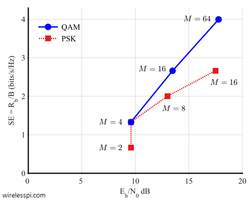
Different constellations with different number of points can be compared by taking all the parameters into account, namely bits/symbol, bandwidth and SNR performance. This can be achieved by plotting the spectral efficiency against the value of $E_b/N_0$ required to obtain a specific target BER. Figure below shows spectral efficiency versus $E_b/N_0$ for QAM and PSK constellations for BER = $10^{-5}$ and excess bandwidth $\alpha = 0.5$, where $E_b/N_0$ values can be taken from the x-axis of BER curves in the previous section. Note that QAM provides better spectral efficiency than PSK because it packs the constellation points in a more efficient manner. This is why it is the modulation of choice in most of the high-speed wireless networks today.
In general, better modulations operate at high spectral efficiency and low $E_b/N_0$, i.e., to the top left of this curve.

On a final note, we rewrite Eq \eqref{eqCommSystemEbNo} here.
\begin{equation*}
\frac{E_b}{N_0} = \frac{P_M}{P_w} \cdot \frac{B}{R_b} = \text{SNR} \cdot \frac{B}{R_b}
\end{equation*}
The above equation can be written as
\begin{equation*}
\text{SE} = \frac{R_b}{B} = \frac{\text{SNR}}{E_b/N_0}
\end{equation*}
As a result, SE can also be seen as the ratio of SNR to $E_b/N_0$. Thus, the lesser $E_b/N_0$ a modulation scheme requires for a given error rate, the more spectrally efficient it is.


If modulation A requires less Eb/N0 than modulation B for a given error rate, modulation A is more power efficient–not more spectrally efficient.
Usually when we say a power efficient modulation, we imply having a lower peak to average power ratio (PAPR) than another modulation for the same average power. It has nothing to do with error rate performance. For example, 16PSK is more power efficient than 16QAM but latter is more spectrally efficient (as shown in the spectral efficiency plot in the last figure above, draw a straight horizontal line between the two points).
Figure shows the Shannon limit on a plot of bit rate vs. signal to noise ratio(E/N). on this plot, QSK and BPSK lie on the same vertical line i.e. they have the same x-axis (E/N) value. Why is this so, and why then would BPSK ever used?
For a given bit rate and a given signal power, QPSK symbol interval is twice as long as that of the BPSK. Since similar energy is available per unit time (definition of power), bits have same energy and both BPSK and QPSK have the same BER. However, for the same symbol rate, BPSK is 3 dB better in link SNR due to no division of energy between two bits.
If we want to achieve a target data rate, we can increase bandwidth to accommodate a higher symbol rate for a fixed power. But do this not still result in an increase in bit error rate because the energy per bit decreases for fixed power and increasing bit rate. Also increasing bandwidth results in a higher received noise power, which further increases probability of error.
So just by increasing bandwidth to accommodate increase in symbol rate, we do not avoid an increase in bit errors
Thanks for the great post! Can we gather any insights on “block error rate” of say, a 16-QAM constellation just from theory?
There are different ways to handle block error rates which would fall outside the scope of this article. I will keep that in mind for a future post though. Thank you.