When I started my PhD, one of the first papers I read was On Maximum Likelihood Estimation of Clock Offset by Daniel Jeske [1] from University of California, Riverside. It eventually set the direction of my future research and ultimately my PhD dissertation. I found this paper quite interesting as it talked about the estimation of clock phase offset. Later I went on to explore what was missing here (the clock frequency offset) and more.
Keep in mind that carrier phase estimation is a different problem that has already been discussed in the past here, here and here. Most of the solutions involve a Phase Locked Loop (PLL) from a software defined radio perspective. In this article, I summarize the main idea of clock offset estimation in simple words.
What is a Timestamp?
The timer in a typical embedded device consists of a counter and a register. Driven by an oscillator, the value of the counter increments or decrements at regular intervals.
- An increment counter typically starts at 0x0…00. When this counter reaches the maximum value of 0xF…FF, it overflows to 0x0…00 and starts counting again.
- On the other hand, a decrement counter typically starts at 0xF…FF. When this counter reaches the minimum value of 0x0…00, it underflows to 0xF…FF and resets the process.
At any instant, e.g., a message arrival event driven by a Rx start interrupt, the value of the counter can be captured and stored in a register that can be later accessed to find the time of that event – according to the node’s own reference clock.
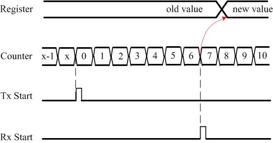
As an example, consider the figure below where
- the timestamp value is captured in Register
- the Counter is an incremental counter
- Tx Start is an event that resets the counter, and
- Rx Start is an event that captures the Counter value to Register.
Timing Exchange
Assume that two nodes exchange above timestamps with each other through the wireless medium as shown in the figure below.
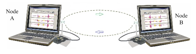
The distance between the two nodes is $R$ while the time of flight from one node to another is $\tau$. Consequently,
$$R = \tau \cdot c$$
We denote the real time by $t$, Node A’s time by $T_A$ and Node B’s time by $T_B$. Since each node starts at a random time, there is a clock offset between its time as compared to the real time. Let us denote the time offset of Node A as $\phi_A$ while that of of Node B as $\phi_B$.
$$T_A = t + \phi_A$$
$$T_B = t + \phi_B$$
Refer to the next figure to observe how the chain of events unfolds.
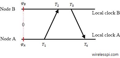
The timestamp exchange process is as follows.
- Node A sends its local timestamp $T_1$ to Node B at real time $t_1$, where
- Node B receives this packet at real time $t_2$ and records its local time $T_2$, where
$$T_2 =t_2 + \phi_B$$
Clearly,
$$t_2 = t_1 + \tau,\qquad or \qquad \tau = t_2-t_1$$
Therefore, we can write
\[
U = T_2-T_1 = t_2 +\phi_B- t_1-\phi_A
\]With $\tau$ as defined above, this can be written as
\[
U = \tau +\phi
\]where $\phi=\phi_B-\phi_A$ is the clock offset between the two nodes.
- After a processing delay, Node B sends its local timestamp $T_3$ at real time $t_3$ to Node A.
- Node A records it at $T_4$ at actual time $t_4$. Since $t_4 = t_3+\tau$,
\[
V = T_4 -T_3 = t_4+\phi_A – t_3 – \phi_B
\]Again, the above expression can be written as
\[
V = \tau ~-~ \phi
\]Next we turn towards the delay distribution encountered in real situations.
Delay Distribution
The above equations were for an ideal scenario of a deterministic clock offset only. In practice, any timing exchange involves random delays that can be incorporated in the above equations as
$$\begin{equation}
\begin{aligned}
U_i ~&=~ \tau + \phi + X_i \\
V_i ~&=~ \tau \,-\, \phi + Y_i
\end{aligned}
\end{equation}\label{equation-model}$$where $X_i$ and $Y_i$ are random delays in the forward and reverse directions, respectively. In the paper, these are modeled as coming from an exponential distribution with mean $\lambda$. This makes sense because delays are never negative. The probability distribution function (pdf) of an exponential random variable is defined as
\[
\nonumber f(x) = \left\{
\begin{array}{l l}
\lambda e^{-\lambda x} & \quad x > 0\\
0 & \quad \textrm{otherwise}
\end{array} \right.
\]With the unit step function defined as
\[
\nonumber u(x) = \left\{
\begin{array}{l l}
1 & \quad x \geq 0\\
0 & \quad \textrm{otherwise}
\end{array} \right.
\]the pdf can be written concisely as
\[
f(x)= \lambda e^{-\lambda x} u(x)
\]Now a maximum likelihood estimate for this delay distribution can be found as follows.
Maximum Likelihood Estimation
Based on the set of $N$ observations $U_i$ and $V_i$ in Eq (\ref{equation-model}), the likelihood function can be written as
\[
L(\tau,\phi) = \lambda^{2N} e^{-\lambda \left( \sum_{i=1}^N U_i + \sum_{i=1}^N V_i- 2N\tau\right)}\cdot u\left(U_{(1)}\ge \tau + \phi~;~ V_{(1)}\ge \tau – \phi\right)
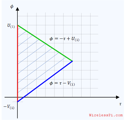
\]where $U_{(1)}$ denotes the minimum value among the observations $U_i$ and $V_{(1)}$ is defined in a similar manner. The terms in the unit step function arise from the respective definitions of $U_i$ and $V_i$ before and the positive nature of the exponential distribution. These two conditions define the region in which likelihood function exists.
\[
\begin{aligned}
\phi &\le -\tau + U_{(1)}\\
\phi &\ge +\tau \,-\, V_{(1)}
\end{aligned}
\]This is shown in the figure below.

Without going into more details (e.g., considering the signs of $U_{(1)}$ and $V_{(1)}$), we can simply infer from the likelihood function that it attains a maximum at the largest value of $\tau$ (as it appears in the exponential of the likelihood function). From the above figure, this is achieved at the right corner of the triangle: at the intersection of the two lines.
\[
-\tau + U_{(1)} = \tau \,-\, V_{(1)}
\]This intersection yields the maximum likelihood estimate of delay as
\[
\hat \tau = \frac{ U_{(1)} + V_{(1)}}{2}
\]By plugging this value back in any one of those equations, we get the maximum likelihood estimate of the clock offset as
\[
\hat \phi = \frac{ U_{(1)} – V_{(1)}}{2}
\]Interestingly, this is the same expression suggested in [2] by informal arguments and empirical observations. This beautiful geometrical derivation kept me interested in exploring the field of synchronization in significant depths during and after my PhD years.
References
[1] D. Jeske, On Maximum Likelihood Estimation of Clock Offset, IEEE Transactions on Communications, Vol. 53, No. 1, Jan 2005.
[2] V. Paxson, On Calibrating Measurements of Packet Transit Times,” Proc. 7th ACM Sigmetrics Conference, Vol. 26, Jun 1998.
$$T_1 = t_1 + \phi_A$$