In major cellular and wireless networks today, space diversity is employed with the help of multiple Tx antennas and/or multiple Rx antennas giving rise to Multiple Input Multiple Output (MIMO) systems. There are three different modes in which multiple antennas can be deployed:
- Beamforming
- Spatial Multiplexing
- Space-Time Coding
In this article, we discuss space-time coding that achieves Tx diversity through multiple antennas at the Tx and simple linear processing at the Rx. This simplicity made this technique quite suitable for the past generations of cellular and other infrastructure based networks. There are two main kinds of space-time codes: Space-Time Block Codes (STBC) and Space-Time Trellis Codes (STTC). In general, STTC offer a better performance than STBC at a cost of increased computational complexity.
Let us start with a very simple scenario in which multiple antennas cannot be used for increased reliability, thus setting the stage for space-time codes.
A Multiple-Input Single Output (MISO) System
In a Multiple-Input Single Output (MISO) system, assume that there are 2 Tx antennas available and only a single Rx antenna as shown in the figure below.

The signal arriving from each Tx antenna is denoted by $r_i$ while the flat fading channel gain is written as $h_i$. Furthermore, since our focus is on one symbol, we can temporarily remove the time index $m$ and denote the data symbol by $s$ only (instead of $s[m]$). Now from the above figure, it is evident that the nature adds the signals impinging at the single Rx antenna allowing us to write
$$ \begin{equation}
\begin{aligned}
r = h_1\cdot s + h_2\cdot s + \text{noise} &= (h_1+h_2)s + \text{noise} \\
&= h\cdot s + \text{noise}
\end{aligned}
\end{equation}\label{equation-miso-1}$$
The channel gains $h_1$ and $h_2$ are complex Gaussian random variables with uniformly distributed phases between $0$ and $2\pi$. Their sum also follows a Gaussian distribution with a uniform phase, i.e., $h=h_1+h_2$. We are facing a similar situation as a simple Rayleigh fading wireless channel! The conclusion is that there is no diversity gain in this setup.
Maximum Ratio Transmission (MRT)
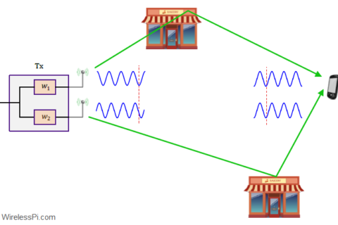
A block diagram of an alternative scheme known as Maximum Ratio Transmission (MRT) for $2$ Tx antennas and $1$ Rx antenna is drawn in the figure below.

Here, the modulation symbol $s$ is weighted by $w_1$ and $w_2$ before sending it through the first and second Tx antennas, respectively. Nature adds these signals at the Rx antenna and the result can be expressed as
\[
r = w_1\cdot h_1\cdot s + w_2\cdot h_2\cdot s+ \text{noise} = \left\{w_1\cdot h_1+w_2\cdot h_2\right\}\cdot s + \text{noise}
\]
Clearly, if we choose random and fixed $w_i$, their sum would neither cancel the phases nor grade the magnitudes according to the channel coefficients $h_i$. The solution is that the modulation symbol $s$ must be weighted by $w_i$ in each branch such that the natural summation at Rx antenna coherently adds electromagnetic energy emanating from each Tx antenna. This can be accomplished by implementing the same solution as in the case of Maximal Ratio Combining (MRC). The idea is that each weight $w_i$ should cancel the phase of the corresponding $h_i$ while contributing to the final summation in proportion to how large that $h_i$ is. This can be achieved through choosing the optimal weights $w_i$ as complex conjugates of channel gains $h_i$.
\[
w_i = h^*_i
\]
A complex conjugate reverses the sign of the $Q$ or imaginary part while leaving the $I$ or real part intact. When optimal $w_i$ are chosen, the signal at the Rx antenna becomes
\begin{equation}\label{equation-mrt}
r = \left\{h_1^*\cdot h_1+h_2^*\cdot h_2\right\}\cdot s + \text{noise} = \Big\{ |h_1|^2+|h_2|^2\Big\}\cdot s + \text{noise}
\end{equation}
The improvement as compared to Eq (\ref{equation-miso-1}) lies in the multiplicative factor with the modulation symbol $s$. While previously it was a fading coefficient $h$ that was the sum of $h_1$ and $h_2$ that could potentially bring each other down, now the factor appearing with data symbol $s$ is $|h_1|^2+|h_2|^2$. This is the best we can do in scavenging the energy from the arriving waves where not only they are being weighted according to the channel gains $h_i$ but also magnitude squared operation prevents any cancelation between their phases.
Separation in Space vs Separation in Time
The above solution seems easy but to choose optimal $w_i$, we must know the channel gains $h_i$ at the Tx. While possible, this is not a straightforward task. Can this Tx diversity of $2$ (or higher) be achieved without any channel knowledge at the Tx? To find the solution, we must recognize the original problem in Tx diversity.
The fundamental problem of Tx diversity is that the two arriving signals automatically add at the Rx without any opportunity to weigh them individually by $w_1$ and $w_2$ at the Rx.
What can be done to avoid this automatic summation by nature at the Rx antenna? One possible trick is to employ more than one time interval for transmission! Now the Rx gets an opportunity to weigh the signal at $T=1$ with $w_1$ and the signal at $T=2$ with $w_2$. Assume that the same modulation symbol $s$ is transmitted in two time intervals as illustrated in the figure below. In communications jargon, this time $T$ is known as a symbol time.

Time Interval 1
The first antenna sends $s$ while the second antenna stays quiet. The Rx signal is given by
\begin{equation}\label{equation-miso-2}
r_1 = h_1\cdot s +\text{noise}
\end{equation}
Time Interval 2
The second antenna sends $s$ while the first antenna stays quiet. The Rx signal is given by
\begin{equation}\label{equation-miso-3}
r_2 = h_2\cdot s +\text{noise}
\end{equation}
Compare the above two equations with a scenario where we had $1$ Tx and $2$ Rx antennas. They are exactly the same! Now we have the opportunity to weigh $r_1$ by $w_1$ and $r_2$ by $w_2$ with their values chosen like MRC.
\[
w_i = h^*_i
\]
We can claim that the error rate of this method is equal to the case of $1$ Tx and $2$ Rx antennas. Hence we have succeeded in achieving a diversity order of $2$ from $2$ Tx and $1$ Rx antennas as well.
Alamouti Scheme
The cost of our first attempt to replicate MRC was the requirement to know the channel gains at the Tx. While we overcame that limitation in the above setup, what is the price paid this time? It is the data rate! Notice that the same modulation symbol $s$ is being sent in two time intervals now, reducing the data rate to half of its previous value. We conclude that diversity with multiple Tx antennas can be achieved as a trade-off with the data rate. Can we restore the information rate while decreasing the error rate through diversity at the same time? This is what space-time coding sets out to achieve. Here, we describe space-time block codes with the help of the first and most well-known example: the Alamouti code.
You can understand Alamouti space-time code easily if you can solve the following set of equations for two numbers $s_1$ and $s_2$.
\begin{align*}
2\cdot s_1 + 7\cdot s_2 &= -1 \\
4\cdot s_1 – 5\cdot s_2 &= 17
\end{align*}
Multiply the first equation with $2$ and subtract the second equation.
\[
19\cdot s_2 = -19
\]
The result is $s_2=-1$ and $s_1=3$. This is quite close to how Alamouti code works.
A hint towards building a space-time code comes from Eq (\ref{equation-miso-2}) and Eq (\ref{equation-miso-3}). There, observe that the second antenna transmits nothing during the first time interval while the first antenna keeps silent during the second time interval. These gaps in transmissions can be efficiently utilized to build a code as follows.
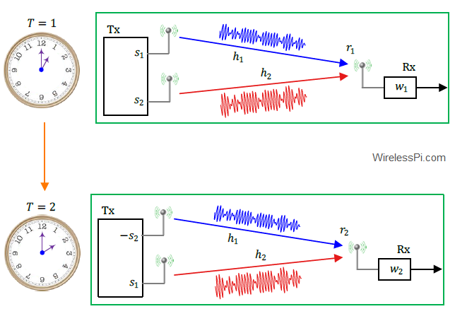
Consider an $N_{\text{Tx}}=2$ and $N_{\text{Rx}}=1$ MIMO system as shown in the figure below. Here, the transmission is divided into two time intervals again.
Time Interval 1
A real modulation symbol $s_1$ (such as from a BPSK constellation) is sent from the first antenna while another real modulation symbol $s_2$ is simultaneously transmitted from the second antenna.
\begin{equation}\label{equation-real-1}
r_1 = h_1\cdot s_1 + h_2 \cdot s_2 + \text{noise}
\end{equation}
The purpose is to achieve a data rate of one symbol per transmission interval as we see next.

Time Interval 2
This is where things get interesting. The trick is to provide in the second interval another reading to the set of equations but with different coefficients. After all, this is how we were able to solve the simple example of the two equations above. Look at the second interval shown as $T=2$ in the figure above where the first antenna sends $-s_2$. The second antenna simultaneously transmits $s_1$. Assuming that the channel gains $h_1$ and $h_2$ stay the same as at $T=1$,
\begin{equation}\label{equation-real-2}
r_2 = -h_1\cdot s_2 + h_2 \cdot s_1 + \text{noise}
\end{equation}
As opposed to the first time interval, this second equation has different coefficients now because $-s_2$ is multiplied with $h_1$, and vice versa!
Combining at the Rx
As shown in the figure above, the weights $w_i$ can now be applied to separate observations $r_1$ and $r_2$ in Eq (\ref{equation-real-1}) and Eq (\ref{equation-real-2}), respectively. Also, the optimal weights $w_i$ are quite similar to MRC or MRT above, $w_i = h^*_i$ but in an alternative manner.
\begin{equation}\label{equation-real-stbc}
\begin{aligned}
w_1\cdot r_1 ~~\xrightarrow~~~ h_1^*\cdot r_1 &= h_1^*\Big\{ h_1\cdot s_1 + h_2 \cdot s_2 + \text{noise} \Big\}\\
w_2\cdot r_2 ~~\xrightarrow~~~ h_2^*\cdot r_2 &= h_2^*\Big\{-h_1\cdot s_2 + h_2 \cdot s_1 + \text{noise} \Big\}
\end{aligned}
\end{equation}
To cancel the cross terms, we take the conjugate of the second equation above. Keeping in mind that modulation symbols are real, i.e., $s_1^*=s_1$ and $s_2^*=s_2$, this leads to
\begin{equation*}
\begin{aligned}
h_1^*\cdot r_1 &= \underbrace{h_1^*\cdot h_1}_{|h_1|^2}\cdot s_1 + h_1^*\cdot h_2 \cdot s_2 + \text{noise} \\
\left\{h_2^*\cdot r_2\right\}^* &= -h_2\cdot h_1^*\cdot s_2 + \underbrace{h_2\cdot h_2^*}_{|h_2|^2} \cdot s_1 + \text{noise}
\end{aligned}
\end{equation*}
The sum of the above two equations cancels the cross terms and sets the modulation symbol $s_1$ free from the influence of $s_2$.
\begin{equation}
z_1 = h_1^*\cdot r_1 + h_2\cdot r_2^* = \Big\{|h_1|^2 + |h_2|^2 \Big\}\cdot s_1 + \text{noise}
\end{equation}
Similar to MRC, the symbol estimate $\hat s$ can be written as
\[
\hat s_1 = \frac{z_1}{|h_1|^2+|h_2|^2}
\]
For known normalized channel gains and a zero noise scenario, this estimate $\hat s_1$ maps exactly on one of the modulation symbols. When noise or other distortions are present, $\hat s$ gets pulled to the nearest constellation point for a decision. Finally, $s_2$ can also be found along similar lines by
\begin{equation}
z_2 = h_2^*\cdot r_1 – h_1\cdot r_2^* = \Big\{|h_1|^2 + |h_2|^2 \Big\}\cdot s_2 + \text{noise}
\end{equation}
and written as
\[
\hat s_2 = \frac{z_2}{|h_1|^2+|h_2|^2}
\]
As you can see, full contributions from $h_1$ and $h_2$ are combined for the decisions on $\hat s_1$ and $\hat s_2$ which like MRC achieves a diversity order of $2$. A few comments are in order here.
Complex Modulation
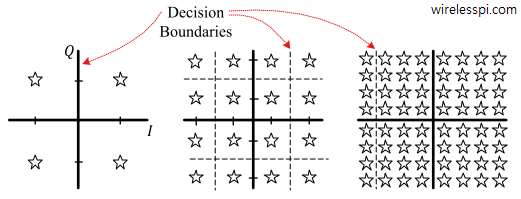
In practice, higher-order modulation schemes such as 4-QAM, 16-QAM and 64-QAM are more often used in wireless networks. Cellular networks employ up to 256-QAM while backhaul microwave links and new generations of WiFi 6 (802.11ax) even use 1024-QAM for faster transmission speeds. QAM stands for Quadrature Amplitude Modulation in which information is sent as complex numbers, the real part on a cosine carrier and imaginary part on a sine carrier. You can learn more about QAM here, here and here.
A block diagram for this case is drawn in figure below. At $T=1$, 16-QAM modulation symbols $s_1$ and $s_2$ are simultaneously sent from the first and second antenna, respectively.

In the second interval shown as $T=2$, the first antenna sends $-s_2^*$. From the definition of a complex conjugate (for a complex number $s=s_I+js_Q$, the complex conjugate is defined as $s^*$ $=$ $s_I – js_Q$. Therefore $-s^*$ $=$ $-s_I + js_Q$), the conjugate of a complex number inverts the sign of the $Q$ or imaginary part, and the negative conjugate of a complex number inverts the sign of the $I$ or real part, i.e.,
\begin{equation*}
\{s^*\}_I = s_I~~\text{and}~~ \{s^*\}_Q = -s_Q \qquad \qquad \{-s^*\}_I = -s_I ~~ \text{and} ~~ \{-s^*\}_Q = s_Q
\end{equation*}
At $T=2$ in figure above, $-s_2^*$ is the bottom right symbol because $s_2$ during $T=1$ was the bottom left symbol in 16-QAM modulation (i.e., only $I$ or real part is inverted). The second antenna simultaneously transmits $s_1^*$ so that $I$ or real part stays unchanged while $Q$ or imaginary part is inverted as compared to $s_1$ during $T=1$. The purpose is not only to provide two equations to the system for solving two unknowns ($s_1$ and $s_2$) but also to provide full diversity for both of the symbols. This was the actual space-time block code proposed by Alamouti. The rest of the details remain the same as the real case above.
Remarks
Some relevant comments are now in order.
Channel Information: In the above derivation, observe that knowledge of channel gains is assumed at the Rx, i.e., $h_1$ and $h_2$ are already known. As mentioned before, this is accomplished in practice by inserting a training sequence or periodic pilot symbols in the information stream (for example, if a starting symbol $s$ is known, the channel gain be estimated from the received signal $r=h\cdot s$ as $\hat h = r/s$).
Complexity: The separation of $s_1$ from interference of $s_2$ and vice versa implies that optimal decisions about $s_1$ and $s_2$ can be taken separately instead of jointly (I deliberately avoid the dreadful `o’ word here: orthogonality). The benefit is that the decoding complexity at the Rx is significantly reduced. The linear combiner used here is both simple and optimal.
Diversity Order: Observe from the detected symbols expressions that the scaling factor $|h_1|^2+|h_2|^2$ is bringing energy from all the Tx branches to provide full spatial diversity of order $2$. Compare this with Eq (\ref{equation-mrt}) for the MRT scheme which also provides full diversity gain of $2$ at the Rx side. The resulting SNR is given by
\begin{equation}\label{equation-snr-alamouti}
\text{SNR}_{\text{Alamouti}} = \frac{1}{2}\cdot\frac{\sum_{i=1}^{2}|h_i|^2}{\sigma^2}
\end{equation}
where $\sigma^2$ is the noise power as before and a normalized power of $1$ is assumed for the symbol $s$. The factor of $1/2$ arises because each signal is sent in two time intervals, once at $T=1$ and again at $T=2$. For the sake of a fair comparison with Rx diversity case where each symbol was sent with unit Tx power $E_s=1$, the Tx power here should then be halved in each interval so that the total Tx power per modulation symbol in those two time intervals stays at $1$.
3 dB Penalty: This translates to a $10 \log 2 \approx 3$ dB power penalty paid for the removal of spatial interference from the other modulation symbol.
Summary
In summary, the Alamouti scheme performs beamforming in time (yes, beamforming) by adjusting the weights $w_i$ in time domain instead of the usual spatial domain. Here, we saw that equipped with $N_{\text{Tx}}=2$ and $N_{\text{Rx}}=1$ antennas, it achieves the same data rate and diversity order as an MRC (or MRT) diversity scheme with $N_{\text{Tx}}=1$ and $N_{\text{Rx}}=2$ antennas. Nonetheless, there is a $3$ dB power penalty for sending the same modulation symbol in two time intervals.
Space-time coding makes data transmission in MIMO systems more reliable but can multiple antennas be instead used to increase the data rates? This is what we do in spatial multiplexing, a topic that is explored in another article.

Thanks for a very nice article.
h1 and h2 are channel gains.
For Eq (7), multiplication with h1* and h2* is done.
How to we estimate h1 and h2 in actual implementation?
This is done through a channel estimation process. Some algorithms for this purpose are quite simple while others are more complicated. In modern wireless systems, this is done through embedding pilot symbols at periodic intervals within the data stream such that the Rx can estimate the channel by knowledge of data. For example, in a flat fading scenario y = h.x, if x is known, then the simplest method for finding h is y/x.
Thank you for this article, it is the best explanation of Alamouti code that I’ve seen. It answers all my misunderstandings. Great Job.
Glad that you liked it. I didn’t find any article or book where space-time codes are explained as beamforming in time (separation in time) with the same underlying SNR-maximizing feature of Maximum Ratio Combining, which is why I wrote this article.
Easy to follow book.
Please could you send me a soft copy of it.
Thanks.