Digitial Signal Processing (DSP) plays a crucial role in algorithm implmentation for building digital and wireless communication systems. A common theme in all those algorithms is that they can be implemented with the following simple operations:
- addition
- multiplication
- shift
In fact, these are the basic principles on which a digital signal processor is constructed. However, when it comes to implementation of real-time systems in hardware such as FPGAs, we find ways to reduce the complexity even further. Which operation (out of the above three) do you think is the most demanding in computations? It is the multiplications.
Therefore, it is preferred to implement signal processing operations in which no multiplications are involved. For example, see the article on spectral translation by half or quarter sample rate and Cascaded Integrator Comb (CIC) filters without any multiplications. Similarly, rotating a complex signal by a certain phase as shown below that helps in carrier phase synchronization can be accomplished through more efficient alternatives. Coordinate Rotation Digital Computer (CoRDiC), invented by Jack Volder in 1956, is one such algorithm that accomplishes this task in a very elegant manner.

Interestingly, the CoRDiC algorithm can implement not only the phase rotations but other operations such as finding the four-quadrant inverse tangent (commonly known as atan2( ) in numerical computing platforms), or polar to rectangular coordinates conversion as well. This is why it is widely used in software defined radios. Let us explore how it works.
Background
In signal processing applications in general and digital communication systems in particular, it is advantageous to work with complex signals that associate the phase of a single sinusoid (e.g., a cosine) with amplitudes of two sinusoids, a cosine and a negative sine. Using the identity $\cos(\alpha+\beta)=\cos \alpha\cdot \cos \beta – \sin \alpha \cdot \sin \beta$, we have
\[
\begin{aligned}
\cos (\omega t +\theta) ~=&~ \cos \omega t \cdot \cos \theta ~-~ \sin \omega t\cdot \sin \theta \\
=&~ \underbrace{\cos \theta}_{\text{amplitude}}\cdot \underbrace{\cos \omega t}_{\text{zero-phase sinusoid}} + \underbrace{\sin \theta}_{\text{amplitude}}\cdot \underbrace{-\sin \omega t}_{\text{zero-phase sinusoid}}
\end{aligned}
\]
This was a simple example of a real sinusoid. Things are a little more complicated when we are dealing with complex signals. What exactly is the expression for a phase rotated complex sinusoid?
\[
\begin{aligned}
\cos (\omega t+\theta) &= \cos \omega t\cdot \cos \theta – \sin \omega t \cdot \sin \theta \\
\sin (\omega t+\theta) &= \sin \omega t \cdot \cos \theta + \cos \omega t \cdot \sin \theta
\end{aligned}
\]
Again, we have a phase shifting of a complex sinusoid in the form of simple amplitude multiplications with $\cos \theta$ and $\sin\theta$. Going further, CoRDiC even eliminates the multiplication operations for phase rotation leaving only simple addition and shift operations.
Rotating a Complex Number
For ease of exposition, we take a complex number $z_0=(x_0,y_0)$ instead of a complex signal as above. Our target is to rotate $z_0$ in a counterclockwise direction by a positive angle $\theta$. The resultant point on the complex plane in this case is given by $z_N=(x_N,y_N)$ where we soon find out the logic behind the subscript $N$. If you know about this neat view of complex numbers, the rotation by $\theta$ is simply a multiplication by $e^{j\theta}$.
\[
z_N = z_0\cdot e^{j\theta}
\]
which can be broken down by using $z_0=x_0+jy_0$ and Euler’s identity $e^{j\theta}=\cos\theta +j\sin\theta$ as
$$\begin{equation}
\begin{aligned}
x_N &= \cos \theta \cdot x_0 – \sin \theta \cdot y_0\\
y_N &= \sin \theta \cdot x_0 + \cos \theta\cdot y_0
\end{aligned}
\end{equation}\label{equation-rotation}$$
There are two tricks that are applied in CoRDiC at this stage.
Breaking Down the Angle
Let us approximate $\theta$ as a sum of $N$ angles (chosen according to a certain criteria coming next).
\[
\theta \approx \sum _{n=0}^{N-1}\theta_n
\]
Since $e^{j\theta}=e^{j\sum _{n=0}^{N-1}\theta_n}$ which are in fact $N$ rotations, we can interpret one rotation by $\theta$ as $N$ rotations in the following sequence.
- $z_0=(x_0,y_0)$ is rotated by $\theta_0$ to yield $z_1=(x_1,y_1)$.
- $z_1=(x_1,y_1)$ is rotated by $\theta_1$ to yield $z_2=(x_2,y_2)$.
- $z_{N-1}=(x_{N-1},y_{N-1})$ is rotated by $\theta_{N-1}$ to yield $z_N=(x_N,y_N)$.
$\vdots$
Similar to Eq (\ref{equation-rotation}), we can write the fundamental recursive equation as
\[
\begin{aligned}
x_{n+1} &= \cos \theta_n \cdot x_n – \sin \theta_n \cdot y_n\\
y_{n+1} &= \sin \theta_n \cdot x_n + \cos \theta_n \cdot y_n
\end{aligned}
\]
for $n=0,1,\cdots,N-1$. Next, the factor $\cos\theta$ can be taken out of all the expressions as
$$\begin{equation}
\begin{aligned}
x_{n+1} &= \cos \theta_n\left(1\cdot x_n – \frac{\sin \theta_n}{\cos \theta_n} \cdot y_n\right)\\
y_{n+1} &= \cos \theta_n\left(\frac{\sin \theta_n}{\cos \theta_n} \cdot x_n + 1 \cdot y_n\right)
\end{aligned}
\end{equation}\label{equation-recursion-with-cosine}$$
Next, we see how to deal with this external scaling factor.
The Scaling Factor $\cos \theta_n$
From hereon, we can ignore the scaling factor $\cos \theta_n$ in further calculations. This is because each $\cos \theta_n$ can be taken out as a separate factor at each step. Therefore, at the end, we have
\[
\cos\theta_0\cdot \cos\theta_1\cdot \cdots \cdot \cos \theta_N
\]
which is a constant number that can be handled only once at the end of the algorithm. Moreover, since $\theta_n$ decreases with $n$ (as we shortly see), the factors after, say $n=5$ or $6$, can be ignored since $\cos \phi \approx 1$ for small $\phi$.
After ignoring $\cos \theta_n$, Eq (\ref{equation-recursion-with-cosine}) can be written as
$$\begin{equation}
\begin{aligned}
x_{n+1} &= x_n – \tan \theta_n \cdot y_n\\
y_{n+1} &= \tan \theta_n\cdot x_n + y_n
\end{aligned}
\end{equation}\label{equation-recursion-without-cosine}$$
This is the expression we use in subsequent operations. Notice that the computational load at each step is two multiplications and two additions. The multiplications can now be cut out by choosing the angles in an intelligent manner.
Choosing the Angles
From fundamentals of digital logic, we know that
- multiplication by a power of two is the same as a left shift of the word by that power, and
- division by a power of two is the same as a right shift of the word by that power.
For example, a number 44 can be represented in binary form as 0010 1100. When it is divided by 4, the answer 11 has a binary representation given by 0000 1011 which is nothing but a right shift of 0010 1100 by 2 places. If we now choose those angles $\theta_n$ (a total of $N$ angles) such that their tangents are powers of 1/2, we can implement the multiplication operations in Eq (\ref{equation-recursion-without-cosine}) as division operations by powers of 2. That leads to their implementation by ordinary left shift operations.
\[
\tan\theta_n = \pm \frac{1}{2^n}
\]
Which angles have tangents as powers of 1/2? You can open a calculator or Wolfram Alpha and verify the following table.

We are now ready to understand the final steps through the help of an example.
A Numerical Example
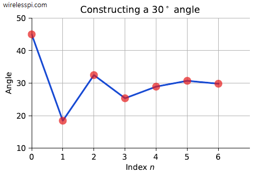
Assume that the complex number $z_0=(x_0,y_0)$ needs to be rotated by an angle $30^\circ$. Using the table above, we can write it as
\[
30^\circ \approx 45^\circ -26.57^\circ+14.04^\circ-7.13^\circ+3.58^\circ+1.79^\circ-0.9^\circ = 29.81
\]
Such a convergence is drawn in the figure below.

How did we determine the sign of each angle in the above equation?
- After the first $45^\circ$, if the marginal sum yields an angle higher than $30^\circ$, a negative sign is attached to the next step so that the rotation should be clockwise or negative towards the final angle.
- On the other hand, if the marginal sum yields an angle lower than $30^\circ$, a positive sign is attached to the next step so that the rotation should be counterclockwise or positive towards the final angle.
Referring to Eq (\ref{equation-recursion-without-cosine}), the final algorithm is given as follows.
\[
\begin{aligned}
x_{n+1} &= x_n \pm \frac{y_n}{2^n}\\
y_{n+1} &= \pm \frac{x_n}{2^n} + y_n
\end{aligned}
\]
where the notation $\pm$ represents a sign that pulls the marginal sum towards $30^\circ$, as explained before.
Computing the Vector Magnitude
You must be wondering why we focus exclusively on the phase rotations above. This is because a number of functions can be calculated through this procedure. As an example, cosine and sine values of an angle can be obtained by starting with $x_0=1$ and $y_0=0$ in Eq (\ref{equation-rotation}).
\[
\begin{aligned}
x_N &= \cos \theta \cdot 1 – \sin \theta \cdot 0 = \cos \theta\\
y_N &= \sin \theta \cdot 1 + \cos \theta\cdot 0 = \sin \theta
\end{aligned}
\]
As another example, suppose that the algorithm starts at a point $z_0=(x_0,y_0)$ and hence the magnitude is given by $\sqrt{x_0^2+y_0^2}$. If this point is rotated towards the x-axis through a negative angle $\theta$, the final point becomes $z_N=(x_N,0)$. Ignoring the constant scaling factor, the magnitude does not change by phase rotation, allowing us to write
\[
\sqrt{x_N^2+0^2}= x_N = \sqrt{x_0^2+y_0^2}
\]
The value $x_N$ is thus the desired result that is quite efficient to compute through this approach. Otherwise, finding the vector magnitude in a digital machine is not an easy task.
Conclusion
We saw how CoRDiC is used to rotate a complex number for phase shifting or de-rotate for a vector magnitude operation. There are several other functions that can be calculated using the same approach such as trigonometric and hyperbolic functions (most importantly, atan2( )), multiplications, divisions, exponentials, logarithms and square roots. This is the reason behind widespread use of CoRDiC in real-time digital signal processing applications. If you are interested, you can also see the intuitive reason behind multiplication and division of complex numbers.