One of the great advantages of Digital Signal Processing (DSP) is an unexpected simplification of operations in seemingly complicated scenarios. See the Cascade Integrator Comb (CIC) filters for how to accomplish the task of sample rate conversion along with filtering with minimal resources.
As another example, in wireless communications and many other applications, a frequency translation is often required in which the spectrum of a signal centered at a particular frequency needs to be moved to another frequency. From the properties of Fourier Transform, a shift by frequency $\omega_0=2\pi F_0$ requires sample-by-sample multiplication with a complex sinusoid $e^{j\omega_0 t}$.
\[
y(t) = x(t)\cdot e^{j\omega_0 t} \qquad \leftrightarrow \qquad X(F-F_0)
\]
In discrete-time, the sampled versions of these signals are
\[
y[n] = x[n]\cdot e^{j\omega_0 nT_S} = x[n]\cdot e^{j\hat \omega_0 n}
\]
where $\hat \omega_0$ is a discrete frequency that is the real frequency normalized by the sample rate $F_S$.
\[
\hat \omega_0 = \frac{\omega_0}{F_S} = 2\pi \frac{F_0}{F_S}
\]
This operation takes significant computational resources. It turns out that this task is significantly simplified for translations by $1/2$ and $1/4$ of the sample rate. Let us explore how.
Translation by Half the Sample Rate $-F_S/2$
We first discuss the sinusoid with frequency $+F_S/2$, examine the impact of its multiplication on the resulting spectrum and then link the result to $-F_S/2$.
The Sampled Sinusoid
In this case, the sampled sinusoid can be written as
\[
e^{j \omega_0 t}\Big|_{F_0=\frac{F_S}{2},~t=nT_S} \qquad \longrightarrow \qquad e^{j2\pi\frac{F_S}{2} nT_S} = e^{j\pi n}
\]
From Euler’s identity $e^{j\theta}=\cos \theta +j\;\sin\theta$, we can write
\[
e^{j\pi n}=\underbrace{\cos (\pi n)}_{(-1)^n} + j\;\underbrace{\sin (\pi n)}_{0} = +1,~-1,~+1,~-1,~+1,~-1,\cdots
\]
Such a signal is drawn at the top of the figure below. An alternating series +1, -1, +1, -1, +1, -1, $\cdots$ is clearly visible. The dotted green line is the underlying continuous-time sinusoid. The half sample-rate frequency is confirmed by the fact that one full period is spanned by only two samples.
\[
T_0 = 2T_S \qquad \longrightarrow \qquad F_0= \frac{1}{2T_S}=\frac{F_S}{2}
\]

The middle figure above is the magnitude spectrum for $N=32$.
- Since the actual frequency is half the sample rate, the discrete frequency is $1/2$ and hence the DFT bin index $k=16$ in a total of $N=32$ spectral samples.
- Since the DFT is periodic with period $N$, the bin $k=16$ is the same as $k=-16$ which is why we can see an impulse at that frequency index and zeros everywhere else. Another way of looking at this periodic nature is that the frequency $-F_S/2$ is the same as $+F_S/2$ in discrete domain.
Finally, the phase spectrum depicts a zero phase for this sinusoid while all zero phases for the remaining values.
The Product Signal
Let us take an example signal $x[n]$ that has a magnitude spectrum shown in the figure below. This signal consists of three sinusoids at bins 10, 11 and 12, respectively. As an exercise for the reader, what are the actual frequencies in terms of the sample rate $F_S$? (Answer: Since $N=32$, these frequencies are $10F_S/32$, $11F_S/32$ and $12F_S/32$, respectively). The phase spectrum is also drawn at the bottom of this figure.

The signal $y[n]$ is a product between the input signal $x[n]$ and the above complex sinusoid.
\[
y[n]=x[n]\cdot e^{j\pi n}
\]
From the nature of $e^{j\pi n}$ described above,
\[
e^{j\pi n} = +1,~-1,~+1,~-1,~+1,~-1,\cdots,
\]
a complex multiplication is not needed anymore. Instead, here is what we do.
- Leave the even-indexed samples of $x[n]$ unchanged.
- Invert the signs of odd-indexed samples.
And this is it. With such an undemanding operation, the whole signal spectrum can be shifted to half the sample rate. This is drawn in the figure below.
- The spectrum centered at bin $k=+11$ can be seen shifted at bin $k=-16+11=-5$.
- The spectrum centered at bin $k=-11$ can be seen shifted at bin $k=-16-11=-27$ that is $k=+5$ after a mod-32 operation.

Let us now look at this concept from a frequency domain viewpoint.
Frequency Domain View
Another way of understanding this spectral shift is the following.
- Multiplication between two signals in time domain is their convolution in frequency domain.
- Moreover, convolution of a baseband signal with an impulse is the signal itself at the location of that impulse.
- The spectral impulse of that complex sinusoid is at $k=-16$.
Combining these results, we can see that the shifted spectrum is just the same as before but centered at $k=-16$ instead of $k=0$.
Translation by Quarter of the Sample Rate $-F_S/4$
Many modern digital communication systems utilize a quarter sample rate translation strategy for efficient downconversion of a wireless signal (owing to a special relationship chosen between Intermediate Frequency (IF) and sample rate). As before, we will discuss the sampled sinusoid first (at frequency $-F_S/4$, not $+F_S/4$) and then examine the impact of its multiplication on the resulting spectrum.
The Sampled Sinusoid
Here, the sampled sinusoid is given by
\[
e^{j \omega_0 t}\Big|_{F_0=\frac{-F_S}{4},~t=nT_S} \qquad \longrightarrow \qquad e^{j2\pi\frac{-F_S}{4} nT_S} = e^{-j\pi n/2}
\]
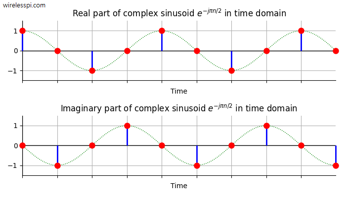
From Euler’s identity $e^{j\theta}=\cos \theta +j\;\sin\theta$, we can write
\[
e^{-j\pi n/2}=\underbrace{\cos (-\pi n/2)}_{+1,0,-1,0,\cdots} + j\;\underbrace{\sin (-\pi n/2)}_{0,-1,0,+1,\cdots}
\]
The real and imaginary parts of this signal are the cosine and sine, respectively. These are drawn in the figure below where alternating series are clearly visible. The dotted green line are their underlying continuous-time versions. The quarter sample-rate frequency is confirmed by the fact that one full period is spanned by only four samples.
\[
T_0 = 4T_S \qquad \longrightarrow \qquad F_0= \frac{1}{4T_S}=\frac{F_S}{4}
\]

Let us examine the magnitude spectrum for $N=32$ shown below. Since the actual frequency is a quarter of the sample rate (with negative sign), the discrete frequency is $-1/4$ and hence the DFT bin index $k=-8$ in a total of $N=32$ spectral samples.

Finally, the phase spectrum depicts a zero phase for this sinusoid while all zero phases for the remaining values.
The Product Signal
Let us observe the spectrum of a signal $y[n]$ that is a product between the input signal $x[n]$ and the above complex sinusoid.
\[
y[n]=x[n]\cdot e^{-j\pi n/2}
\]
From the nature of $e^{-j\pi n/2}$ described above,
\[
e^{-j\pi n/2} = \{+1,~0,~-1,~0,\cdots\} + j\{0,~-1,~0,~+1,\cdots\}
\]
Again, we can see that a complex multiplication is not needed anymore. The whole signal spectrum can be shifted to a quarter of the sample rate through mere signal routing. This spectrum is drawn in the figure below.
- The spectrum centered at bin $k=+11$ can be seen shifted at bin $k=-8+11=+3$.
- The spectrum centered at bin $k=-11$ can be seen shifted at bin $k=-8-11=-19$ that is $k=+13$ after a mod-32 operation.

From a frequency domain viewpoint, the shifted spectrum is just the same as before but centered at $k=-8$ instead of $k=0$.
Implementation
How can you implement the above frequency translations in hardware such as a DSP or FPGA? In case of $F_S/2$ shift, we only need to invert the signs of odd-indexed samples. In the current scenario of $F_S/4$, we need to inspect the real and imaginary parts (or IQ samples) of the product signal.
\[
\begin{align*}
x[n]\cdot e^{-j\pi n/2} &= (x_I + jx_Q)\{\cos (\pi n/2)-j\sin (\pi n/2)\} \\
\\
&= x_I \underbrace{\cos(\pi n/2)}_{+1,~0,~-1,~0,~\cdots}+ x_Q\underbrace{\sin (\pi n/2)}_{0,~+1,~0,~-1,~\cdots} + j \Big\{x_Q \underbrace{\cos (\pi n/2)}_{+1,~0,~-1,~0,~\cdots} – x_I \underbrace{\sin (\pi n/2)}_{0,~+1,~0,~-1,~\cdots}\Big\}
\end{align*}
\]
From here, observe that for the output signal,
- even-indexed samples of $x_I$ and odd-indexed samples of $x_Q$ form the inphase part, and
- even-indexed samples of $x_Q$ and odd-indexed samples of $x_I$ form the quadrature part.
Conclusion
In summary, just by inverting the signs of even and/or odd-indexed samples of $x[n]$, we have managed to move its spectrum from baseband to 1/4 or 1/2 of the sample rate. This demonstrates the unconventional power of DSP.
If you are interested in application of DSP algorithms in communication system design, you can see my book on software defined radios.