In olden days, people used to have lots of kids. A famous Urdu satirist once wrote: "It has been observed that the last kid is usually the most mischievous of them all. Therefore, there should be no last kid in a family!" I remembered this line today because I have observed that starting a write-up is the most difficult task of them all. Therefore, there is no introductory paragraph in this article. Suffice it to say that this is the only topic I have found that takes you from a very small first step (just two additions) to really advanced concepts (filter design, cascades and register growth) in the field of DSP, and hence the staircase in the title.

A Moving Average Filter
Cascaded Integrator Comb (CIC) filters, also known as Hogenauer filters, are an example of the simplest of computations, i.e., a few additions, no multiplications and limited memory storage, performing the most laborious of jobs, i.e., filtering at high sample rates. Their origin lies in a moving average filter.
In the field of digital signal processing, a moving average filter is to other fancy filters what a Forrest Gump is to a room full of Einsteins. It has no more capability than to compute an average of $L$ readings as
\begin{equation}\label{equation-moving-average-1}
y[n] = \frac{1}{L}\Big\{x[n]+x[n-1]+x[n-2]+\cdots + x[n-L+1]\Big\}
\end{equation}
A block diagram of such an operation is drawn in the figure below for $L=5$ where $D$ denotes a delay of one sample. In DSP, this delay is usually denoted by $z^{-1}$. For the sake of simplicity, we will continue with the notation $D$ instead of $z^{-1}$. The cost of implementation can be seen as $L-1$ delays and $L-1$ additions, both of which increase with block length $L$.

There are two ways to characterize any system: an impulse response and a frequency response.
Impulse Response
An impulse response is defined as the output of a system when the input $x[n]$ is a unit impulse $\delta [n]$.
\[
\delta[n] = \left\{ \begin{array}{l}
1, \quad n = 0 \\
0, \quad n \neq 0 \\
\end{array} \right.
\]
This is a single sample with amplitude $1$ at time index $0$. When this is given as an input to the filter in the figure above, it is evident that the impulse response is a sequence of all ones because this same impulse gets shifted to the right at each cycle. This is plotted in the figure below for $L=10$. The shape reveals why a moving average is also known as a rectangular or a boxcar filter.
\begin{equation}\label{equation-cic-boxcar}
h[n] = \left\{ \begin{array}{l}
1, \quad 0 \le n \le L-1 \\
0, \quad \text{otherwise} \\
\end{array} \right.
\end{equation}

This impulse response results in an overall filter gain at DC defined by
\begin{equation}\label{equation-cic-moving-average-gain}
\sum _{n=0}^{L-1} h[n] = \sum _{n=0}^{L-1} 1 = L
\end{equation}
A scaling by $1/L$ is not as important for floating-point simulations but need to be taken into account for fixed-point implementations in hardware.
Frequency Response
The frequency response of a filter shows its behavior with respect to different frequencies. It can be found through the Discrete-Time Fourier Transform (DTFT) of the impulse response.
\[
H\left(e^{j\omega}\right) = \sum_{n} h[n]e^{-j\omega n}
\]
Plugging in the impulse response from Eq (\ref{equation-cic-boxcar}), we get
\[
H\left(e^{j\omega}\right) = \sum_{n=0}^{L-1} 1\cdot e^{-j\omega n} = \sum_{n=0}^{L-1} \left(e^{-j\omega}\right)^n
\]
Using the familiar geometric series formula given by
\[
\sum \nolimits_{n=n_1}^{n_2} a^n = \frac{a^{n_1} – a^{n_2+1}}{1-a},
\]
we can write
\begin{align*}
H\left(e^{j\omega}\right) &= \frac{1 – e^{-j\omega L}}{1 – e^{-j\omega}} = \frac{e^{-j\omega\frac{L}{2}} \left(e^{+j\omega\frac{L}{2}} – e^{-j\omega \frac{L}{2}} \right)}{e^{-j\frac{\omega}{2}}\left(e^{+j\frac{\omega}{2}} – e^{-j\frac{\omega}{2}} \right)} \\
&= e^{-j\omega\frac{L-1}{2}} \cdot \frac{\sin \left(\omega L/2 \right)}{\sin \left( \omega/2\right)}
\end{align*}
where the relation $j2 \sin \theta = e^{+j\theta} – e^{-j\theta}$ is used in the last step. The first term above is the phase part which can be eliminated if the impulse response is centered around $n=0$. The frequency response is now expressed in a more common form by plugging in $\omega=2\pi f$ as
\begin{equation}\label{equation-cic-moving-average-spectrum}
H\left(f\right) = \frac{\sin \left(\pi L f\right)}{\sin \left( \pi f\right)}
\end{equation}
Here, $f$ is the discrete frequency defined as
\begin{equation}\label{equation-discrete-frequency}
f = \frac{F}{f_s}
\end{equation}
where $F$ is the real frequency in Hz and $f_s$ is the sample rate. This sample rate is a crucial but invisible component of this expression that plays an important role in sample rate conversion applications like decimation and interpolation, as we find out later. This magnitude response is drawn in the top subplot of the figure below while the same response in dB is plotted in the bottom subplot.

- At zero Hz or Dc, both the numerator and the denominator are zero and the mainlobe peak can be found by applying L’Hopital’s rule that is the same DC gain found earlier in Eq (\ref{equation-cic-moving-average-gain}).
\[
H(0) = \frac{\cos (\pi L f)\cdot \pi L}{\cos (\pi f)\cdot \pi}\bigg|_{f=0} = L
\]The position of the first null is derived later during the discussion on differential delay where it is more relevant.
- From the spectrum, it is evident that a moving average filter acts like a lowpass filter, i.e., it allows to pass signals at lower frequencies (with some distortion) and it blocks signals at higher frequencies.
- This response, however, is a poor man’s lowpass filter (see the familiar $-13$ dB first sidelobe suppression). And there are no coefficients to control the passband, stopband or transition band parameters. This is a direct result of the simple averaging or addition operation performed without any multiplications.
Such a simple summation does not seem appropriate for the most critical component of a radio transceiver, i.e., the digital frontend. However, in 1981, Eugene Hogenauer [2] (and at least one more person) observed something interesting when this average needs to be taken at each cycle, as explained next.
Recursive Sum
From the previous reading in Eq (\ref{equation-moving-average-1}), we can write
\begin{equation}\label{equation-moving-average-2}
y[n-1] = \frac{1}{L}\Big\{x[n-1]+x[n-2]+\cdots + x[n-L+1] + x[n-L]\Big\}
\end{equation}
Subtracting Eq (\ref{equation-moving-average-2}) from Eq (\ref{equation-moving-average-1}) and ignoring the scaling by $L$ for now, we get
\[
y[n]-y[n-1] = x[n] – x[n-L]
\]
This gives a recursive implementation as
\begin{equation}\label{equation-cic-recursive-sum}
y[n] = x[n] – x[n-L] + y[n-1]
\end{equation}
A block diagram of such a recursive sum is plotted in the figure below for $L=5$. This expression tells us that each newly arriving input $x[n]$ is included in the new sum while $L$-samples old input $x[n-L]$ is excluded. It is evident that the cost of implementation has significantly changed.
- The number of required delay elements has increased to $L+1$ as compared to the moving average filter with $L-1$ delays.
- However, the number of additions has reduced from $L-1$ to just $2$, regardless of the value of $L$! This is a huge saving, particularly for large $L$, that makes this option attractive in high rate systems.

We are ready to transition towards CIC filters now.
How an Integrator and a Comb are Cascaded
A CIC filter in its simplest form is the same as the recursive sum filter drawn in the figure above. When these $L$ delays are represented in a compact form as shown in the figure below, we have our 1st-order $L$-point Cascaded Integrator Comb (CIC) filter.

Where do the labels Comb and Integrator come from? To answer this question, rewrite Eq (\ref{equation-cic-recursive-sum}) as
\begin{align}
y[n] &= \underbrace{x[n] – x[n-L]}_{\text{Comb}~c[n]} + y[n-1] \nonumber \\
&= \underbrace{c[n] + y[n-1]}_{\text{Integrator}}\label{equation-cic}
\end{align}
We begin with the description of the comb filter first. From Eq (\ref{equation-cic}), the comb response can be seen as
\begin{equation}\label{equation-cic-comb-relation}
c[n] = x[n] – x[n-L]
\end{equation}
As with moving average filter, a comb is characterized through an impulse response and a frequency response.
Impulse Response
To find the impulse response of the comb, we simply replace $x[n]$ with $\delta [n]$ in Eq (\ref{equation-cic-comb-relation}).
\begin{equation}\label{equation-cic-comb-impulse-response}
h_c[n] = \delta [n] – \delta[n-L]
\end{equation}
This is drawn in the figure below for $L=10$ where a positive impulse at time $n=0$ and a negative impulse at time $n=10$ can be observed. All the remaining values are zero resulting in no multiplication or addition operations for computing the output.

Frequency Response
Just like the moving average case, we can find the frequency response of a comb filter through the Discrete-Time Fourier Transform (DTFT) of its impulse response. From Eq (\ref{equation-cic-comb-impulse-response}),
\begin{align*}
H_c\left(e^{j\omega}\right) &= \sum_{n} h_c[n]e^{-j\omega n} \\
&= \delta[n]e^{-j\omega n} – \delta[n-L]e^{-j\omega n} = 1 – e^{-j\omega L}
\end{align*}
where we have used the fact that $\delta[n-n_0]$ is $1$ at $n_0$ and zero elsewhere. This can be simplified as follows.
\begin{align*}
H_c\left(e^{j\omega}\right) &= e^{-j\omega \frac{L}{2}}\left(e^{+j\omega \frac{L}{2}} – e^{-j\omega \frac{L}{2}}\right) \\
&= e^{-j\omega \frac{L}{2}} \cdot j2 \sin \left(\omega \frac{L}{2}\right)
\end{align*}
In terms of discrete frequency $f$, we write
\begin{equation}\label{equation-cic-comb-spectrum}
H_c\left(f\right) = e^{-j\pi L f} \cdot j2 \sin \left(\pi L f\right)
\end{equation}
The first term and the factor $j$ contribute towards the phase only and all that is left for magnitude is a sine wave. This frequency domain sine wave is plotted at the top of the below figure for $L=10$ where the negative cycles appear as positive due to the absolute value operation. The middle plot shows the same response in dB. The shape of this curve is the reason behind the term comb because there are $L$ nulls in the frequency response at equally spaced intervals that makes the spectrum look like a thick comb.


Why are there $L$ nulls? Because a sinusoid with frequency $1$ crosses zero twice in one period. This frequency domain sine wave in Eq (\ref{equation-cic-comb-spectrum}) has an inverse period equal to $L/2$ or a period of $2/L$. For $L=10$, this turns out to be $0.2$ within which two nulls appear.
Let us turn our attention towards the integrator now. From Eq (\ref{equation-cic}), the integrator expression can be seen as
\[
y[n] = c[n] + y[n-1]
\]
To find the impulse response, we simply replace the input $c[n]$ with the unit impulse $\delta [n]$. Starting with an initial condition $y[-1]=0$, it is straightforward to see from the above definition that
\[
y[0] = 1+0, \qquad y[1] = 0+1=1, \qquad y[2] = 0+1 =1, \cdots
\]
Therefore, the impulse response of the integrator is given by the unit step signal that is zero for $n<0$ and $1$ for $n\ge 0$.
\[
h_i[n] = u[n]
\]
Such an impulse response is drawn in the middle plot of the below figure. The top subplot shows the comb impulse response from the earlier discussion. From basic DSP theory, the cascade response of two filters in time domain is given by their convolution.
\[
h_{\text{CIC}}[n] = h_c[n]*h_i[n]
\]
The result of this convolution is shown in the bottom plot of the figure below.

Why does this bottom plot resemble the impulse response of a moving average filter? Because the cascade of a comb and an integrator is a moving average filter, see Eq (\ref{equation-cic-recursive-sum}). As far as the convolution is concerned, the positive impulse at time $0$ in the comb starts the integrator’s first output as $1$. Then, the remaining zeros ensure that this $1$ keeps appearing (thanks to the feedback $y[n-1]$) until the negative impulse at time $L$ arrives. From here onward, each such $1$ is canceled by a $-1$ from this last index and the rest of the values are all zero.
Sample Rate Conversion
CIC filters play an integral role in sample rate conversion in the digital frontend of a radio (we have also discussed spectral shifts by a certain amount without any multiplications before). We begin with the scenario of downsampling (also known as decimation) while the upsampling (also known as interpolation) case can be understood through duality between these two operations.
A downsampling operation of a digital signal is quite similar to sampling a continuous-time signal. We need an anti-aliasing filter before the sample rate change to suppress the spectra that would fold into the first Nyquist zone as a result. At high sample rates, a CIC filter can play the role of that anti-aliasing filter for fast processing.
Such an arrangement is drawn in the figure below which is a redrawn version of the recursive sum figure before. Here, the sample rate is converted through an $L:1$ downsampling operation, i.e., $L-1$ samples are thrown away between every two samples. Keep in mind that the downsampling rate $R$ need not be equal to $L$. It could be related to the comb delay $L$ through a parameter known as a differential delay that will be discussed in differential delay explanation. For now, we continue the discussion with $L=R$.

The upsampling operation is the dual of downsampling the signal. For a $1:L$ rate conversion, we insert $L-1$ zeros between every two samples that inserts $L-1$ spectral copies, known as images, of the signal within the same band. Therefore, an anti-imaging filter is required to suppress these spectra as a result, a task efficiently accomplished by a CIC filter. Such an arrangement is the dual of the above figure and hence not drawn here for conciseness. Instead, we just look at the spectra below that appear during the interpolation process. This is because it is straightforward to observe the impact of sample rate change and filtering in this setting. Refer to the figure below and observe the following.

- The top plot is the spectrum of the moving average filter. This is also the spectrum of a CIC filter which is simply an efficient implementation of a moving average filter. Notice how the x-axis is now scaled by $L=10$ in this case since $f$ is defined according to the input sample rate.
- The middle plot displays the spectrum of an upsampled signal that is obtained through stuffing $L-1$ zeros between every two samples of input $x[n]$. Such an operation increases the sample rate by a factor of $L$ and gives rise to $L-1$ extra replicas within the higher sample rate at the output. The dashed line in the background represents the CIC filter response from the top plot to verify which parts of the signal spectrum survive after the filtering process.
- The bottom plot illustrates the output signal spectrum after the filtering process. Observe how images of the original spectrum survive at multiples of the input sample rate but their contribution in the output spectrum is determined by the sidelobe suppression of the CIC filter. This is why the high-rate output signal is not a clean copy of the low-rate input signal in this case. In general, two strategies are adopted to clear these remnants, cascading multiple CIC filters in series and one or more conventional FIR filters at the end of the chain.
- Finally, the scenario for decimation is the dual of this process. After sample rate reduction by $L$, a total of $L-1$ spectral remnants from regions around multiples of $1/L$ alias into our signal bandwidth thus distorting the downsampled signal.
The reader would have noticed in the block diagram of the initial decimation filter that comb precedes the integrator. A question then arises why the terminology CIC was not named as CCI. For this purpose, observe in the same figure that the input sample rate is $f_s$ while the output sample rate is $f_s/L$. This implies that the filtering operations are performed at the higher of the two rates. This seems inefficient because $L-1$ out of every $L$ samples are discarded at the filter output which is given as
\[
y[m] = y[nL]
\]
We should not be computing the outputs that are going to be discarded at the very next step. To arrive at a more efficient architecture, notice the following.
- Both the comb and the integrator are linear processes. One of the properties of linear systems is that their order does not matter, i.e., the order in a cascade of two linear systems can be reversed. This is shown in the figure below where the comb and integrator are followed by a downsampler at the end. However, the order of the comb and the integrator can be interchanged due to linearity.
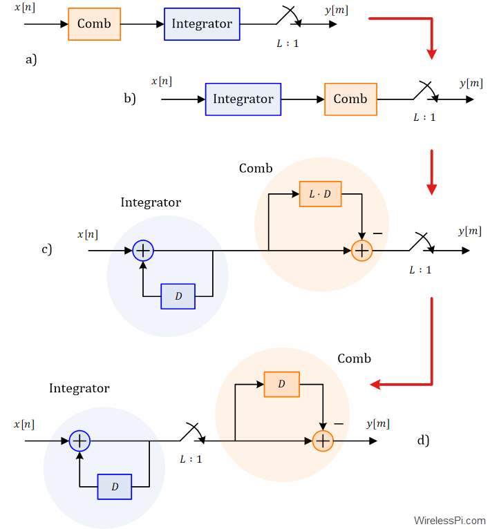
- Next, the actual block diagrams for the integrator and the comb are drawn. Observe that from the viewpoint of the downsampler, computing a comb output through subtraction after a delay of $L$ samples at its input is equivalent to computing the same result through subtraction after a unit delay at the output!
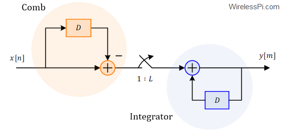
- This implies that the order of the comb and the downsampler can be interchanged as shown at the bottom of the figure. The technical term for this exchange is known as the noble identity. There are two benefits of this arrangement: one, the comb operates at a reduced clock rate, and second, its data storage requirement has reduced from $L$ to just $1$. Now we can see why the terminology CIC mentions the integrator first and the comb second.
- Finally, the block diagram of an interpolation CIC filter for rate $L$ is shown in the figure below. Observe how the comb section operates on the low-rate input samples $x[n]$ before delivering them to the integrator that computes the high sample rate output.


Along with the article, you can get the Matlab/Octave code for a CIC decimating filter chain if you are developing a wireless product or working on a DSP project.
A part of a sample script is shown in the figure below.

Towards Better Stopband Attenuation
The magnitude spectrum of a CIC filter was plotted earlier. From here, we deduce that it is not a particularly good lowpass filter because the peak stopband attenuation (appearing at the first sidelobe) is only $13$ dB below the mainlobe peak. To improve this response, one solution is to cascade multiple CIC filters together to build an order-$N$ CIC filter. A block diagram of this approach is drawn for a multistage decimation CIC filter in the figure below. For $N=3$, three integrators operate on the input signal $x[n]$ before downsampling to a low rate $L:1$. Then, three comb filters operate on the downsampled signal to generate the final output $y[m]$.

We achieve improved stopband attenuation by this technique because joining $N$ linear systems in a series results in an overall system with an impulse response given by the convolution of individual impulse responses. Moreover, convolution in time domain gives rise to multiplication in frequency domain.
\[
\underbrace{h[n]*h[n]*\cdots *h[n]}_{N~\text{times}} \qquad \rightarrow \qquad \left[H(f)\right]^N
\]
Based on this result, we can write the frequency response for an order-$N$ CIC filter from Eq (\ref{equation-cic-moving-average-spectrum}) as
\begin{equation}\label{equation-cic-spectrum}
H_{\text{CIC}}\left(f\right) = \left[\frac{\sin \left(\pi L f\right)}{\sin \left( \pi f\right)}\right]^N
\end{equation}
Such a spectrum is plotted in the figure below for orders $N=1, 2, 3$ and $4$. Owing to the above expression, the first order CIC has a peak sidelobe given by $-13$ dB. With each additional stage, another $13$ dB of attenuation is added to the response (due to the logarithmic scale). This is why the peak sidelobes for $N=2, 3$ and $4$ can be seen as $-26$ dB, $-39$ dB, and $-52$ dB, respectively.

The price we pay for this improved attenuation is the hardware and passband droop, as explained next.
Hardware
Each additional stage requires more adders and delay elements. Furthermore, due to the normalized response, what we cannot see in the above figure is the increasing mainlobe gain. The higher gain at each stages necessitates a larger word width in hardware. This is an issue we handle during the discussion on CIC gain.
Passband Droop
From the shape of the curves in the above figure, notice how the mainlobe gets narrower with each subsequent stage (the null positions stay the same, however). This increased droop makes an order-$N$ CIC filter difficult to implement beyond a certain percentage of the mainlobe width because a signal within the filter passband is shaped by this steep curve too. A good choice for passband edge is below a quarter of the first null at low rate.
Despite these problems, their filtering capability at a very low computational cost necessitates a widespread implementation of multistage CIC filters in digital radio systems and solutions to these problems are found instead.
Role of Differential Delay
Until now, we considered a decimation or interpolation factor equal to the number of delays in the comb section. Due to this reason, the differential delay shown in all the figures was just $1$. This is a common but not necessary practice in digital radio frontends where sometimes a differential delay of $2$ is also employed. We denote this factor by $M$. This means that the comb section consists of $M$ delays instead of $1$. This is drawn in the figure below for a rate change factor $R$.

The filter length $L$ can now be written in terms of the decimate or interpolation rate $R$ as
\[
L = R\cdot M
\]
But why is this factor $M$ needed? In the spectrum of decimation by $L=10$ example, we observed that there are $L-1$ nulls within the response at the input sample rate. The length $L$ determines the number of nulls (and hence the position of the first null and the mainlobe width) that can be found from the magnitude response of the CIC filter in Eq (\ref{equation-cic-moving-average-spectrum}) reproduced below.
\[
H\left(f\right) = \frac{\sin \left(\pi L f\right)}{\sin \left( \pi f\right)}
\]
At $f=0$, both the numerator and the denominator are zero. So the first null corresponds to the next zero-crossing of the numerator sine since its inverse period is $L$ times higher than the denominator. This zero-crossing occurs when the argument of the numerator sine equals $\pm \pi$.
\[
\pi L f_1 = \pm \pi, \qquad \qquad f_1 = \pm \frac{1}{L}
\]
We conclude that the factor $L$ not only controls the DC gain but also the bandwidth of the filter.
Now the differential delay $M$ proves useful in a situation where the upsampling or downsampling factor $R$ is different than the desired filter length $L$ due to the following reasons.
- Placement of nulls at specific locations
- Increased sidelobe attenuation
Turning to the example we are working with throughout this article, i.e., a decimation CIC filter with length $L=10$, assume that the decimation factor $R=5$ and the differential delay $M=1$. The top plot in the below figure shows a wide mainlobe and only $4$ nulls in the spectrum. On the other hand, for the same rate change $R$, increasing the differential delay from $M=1$ to $M=2$ now doubles the locations of nulls. The passband width also gets reduced as evident from the bottom plot.

CIC Gain and Register Growth
Recall from the first section that the gain of a moving average filter is given by $1$ because the coefficients are scaled by $1/L$. However, when it was redesigned in a recursive form, this factor of $1/L$ was removed. It cannot be compensated for at the end due to the bit growth that happens in all the cascaded integrator and comb stages.
- Similar to the gain of an $L$-point moving average filter in Eq (\ref{equation-cic-moving-average-gain}), a 1st-order CIC filter has a gain of $L=RM$ where $R$ is the rate change factor and $M$ is the differential delay. An integrator keeps accumulating the input on the way to infinity and the register contents inevitably overflow. Nevertheless, this intermediate overflow does not cause an error in the final output as long as the following two conditions are met.
- 2’s complement arithmetic is used for sample representation.
- The accumulator (and the subsequent stages) is sufficiently wide to hold the correct result.
What does sufficiently wide mean? Take the example of $R=10$ and $M=1$ where the gain $G=RM=10$. If the input to the decimation CIC filter is $8$ bits wide (i.e., the maximum value is $-2^7=-128$ for signed integers), then all the integrators and combs should be able to hold the maximum input times the gain, or $-128\times 10=-1280$ which is greater than $2^{10}=1024$. For signed case, this requires $12$ bits of precision that can be generalized with the following formula.
\[
B = B_x + \text{ceil}\big[\log_2 RM)\big]
\]Plugging in $B_x=8$, $R=10$ and $M=1$ from the example, $B$ is equal to $8$ plus $4$, or $12$.
- A series of $N$ CIC filters then has a gain of
\[
G = \underbrace{RM\cdot RM \cdots RM}_{N~\text{times}} = (RM)^N
\]This gain exhibited by the order-$N$ decimation CIC filter increases exponentially with $N$. The register width now required for all the stages is
\[
B = B_x + \text{ceil}\big[N\cdot \log_2 RM\big]
\]For a similar example as above, but with $N=4$ stages, the required register width is
\[
B = 8 + \text{ceil}\big[4\cdot \log_2 10\big] = 8 + 14 = 22
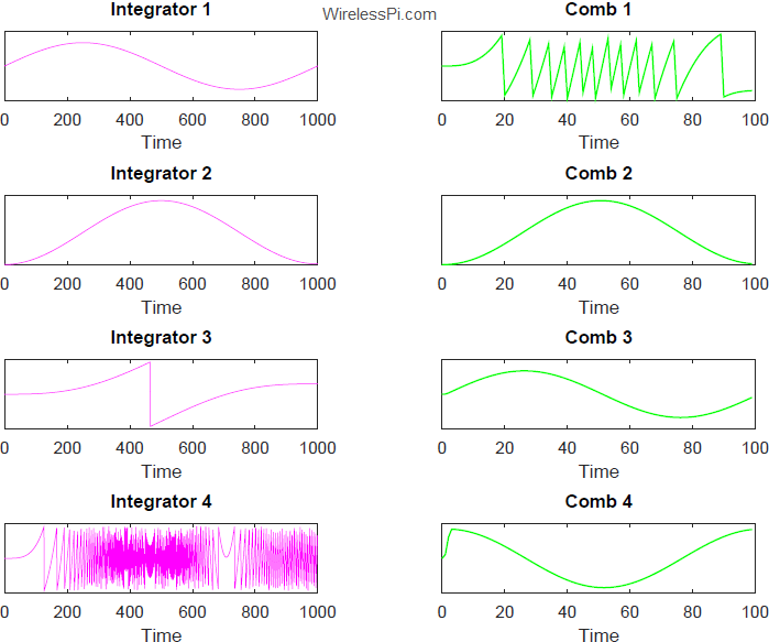
\]We conclude that the initial $8$ bits need to be sign-extended to $22$ bits before the first CIC stage. When 2’s complement arithmetic is used along with sufficiently wide registers, overflows in the integrators do not distort the final output. An example with decimation by $R=10$, $M=1$ and $N=4$ CIC stages is drawn in the figure below. Notice how integrators overflow but then subsequently corrected by the comb stages. Not shown in the figure are the increasing amplitudes on y-axis as a result of processing from the integrators.
- This bit growth is usually truncated at the end of the processing chain that incurs quantization errors in the results. For decimation CIC filters, Hogenauer [2] describes a technique to optimally distribute this truncation between successive CIC stages in such a way that the quantization errors accumulated by this distributed truncation are still the same as one final truncation.
- Since zero stuffing during the upsampling process reduces the output gain by a factor of $R$, an order-$N$ CIC interpolation filter has a gain at the final stage given by
\[
G = \frac{(RM)^N}{R}
\] - Taking into account this gain and following a similar logic as for decimation, the maximum register width for interpolation can be written as
\[
B = B_x + \text{ceil}\big[\log_2 \frac{(RM)^N}{R}\big]
\] - In CIC interpolation filters, truncation or rounding cannot be used because resulting small errors can grow without bound in the integrators. Therefore, each stage of an interpolation CIC filter must use full-precision arithmetic and truncation or rounding can only be applied at the final output.

Designing a CIC Compensation Filter
Typical FIR filters have a relatively flat passband to ensure that a desired signal does not get distorted. While CIC filters do an excellent job of filtering the signals in stopband at a low complexity, their passband droop described earlier and large transition width (the region between passband and stopband) are not desirable from a filtering viewpoint. To understanding this point, recall the shape of the curves in a CIC filter spectrum and observe how the mainlobe gets narrower with each subsequent stage as the null positions stay the same. This increased droop makes an order-$N$ CIC filter difficult to implement beyond approximately a quarter of the mainlobe width because a signal within the filter passband is shaped by this steep curve too.
We describe the solution for a decimation by $L=10$ CIC filter chain, the same example we are working with throughout this article. The scenario for interpolation is simply the dual of this problem. In a practical implementation, $N$ stage integrators and combs are followed by one or more FIR compensation filters that perform the following tasks:
- Compensate for the passband droop
- Sharpen the overall transition region
- Suppress the spectral remnants left over by CIC
- Decimate the CIC output by another factor of $2$, if desired
Let us derive the transfer function of this compensation FIR filter for $L=RM$, where $L$ is the filter length of the underlying moving average filter, $R$ is the decimation factor and $M$ is the differential delay. The starting point is Eq (\ref{equation-cic-moving-average-spectrum}) that is reproduced below. It describes the magnitude response of a length equal to $L=RM$ moving average, and hence CIC, filter.
\[
H\left(f\right) = \frac{\sin \left(\pi RM f\right)}{\sin \left( \pi f\right)}
\]
A point of particular importance is that the discrete frequency $f$ is defined with respect to the higher sample rate, $f_s$, in a decimation filter. Here, $F$ is the real frequency in Hz.
\[
f = \frac{F}{f_s}
\]
This can cause a misunderstanding in actual filter design because it needs to be designed for lower rate $f_s/R$ while the CIC passband droop exists according to the magnitude response of the higher rate $f_s$.
Next, after plugging this discrete frequency value in the magnitude response, we get the expression in terms of real frequency $F$.
\[
H\left(F\right) = \frac{\sin \left(\pi RM \frac{F}{f_s}\right)}{\sin \left( \pi \frac{F}{f_s}\right)} = \frac{\sin \left(\pi M \frac{F}{f_s/R}\right)}{\sin \left( \pi \frac{F}{R (f_s/R)}\right)}
\]
We arrive at our final expression in terms of the discrete frequency $f’=F/(f_s/R)$, i.e., the one normalized by the output sample rate $f_s/R$.
\[
H\left(f’\right) = \frac{\sin \left(\pi M f’\right)}{\sin \left( \pi f’/R\right)}
\]
This is the passband droop that needs to be corrected in the low rate FIR compensation filter. A widely used technique is to simply invert this response to get the filter transfer function $H_{CF}(f’)$ that also includes the contribution from the number of CIC stages $N$.
\begin{equation}\label{equation-cic-decimation-spectrum}
H_{CF}\left(f’\right) = \left[\frac{\sin \left( \pi f’/R\right)}{\sin \left(\pi M f’\right)}\right]^N
\end{equation}
There are two scenarios to be considered here, wideband compensation and partial band compensation.
Wideband Compensation
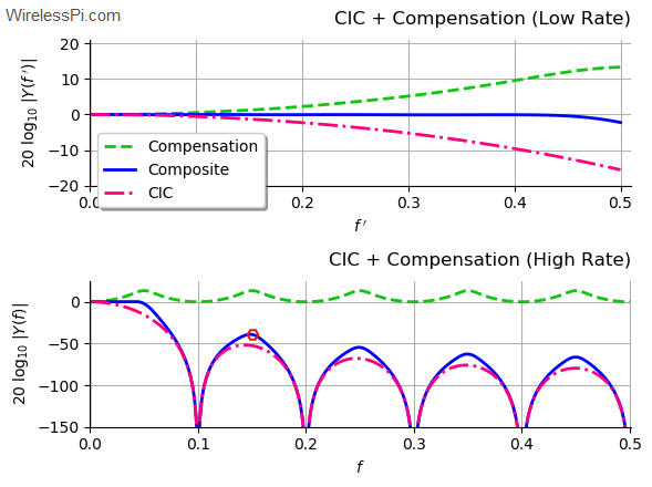
When the signals of interest can lie anywhere in the passband region at the low sample rate $f_s/R$, a wideband compensation FIR filter needs to be employed that compensates for the droop over the whole region from $-f_s/(R/2)$ to $f_s/(R/2)$ (due to the symmetry of the spectrum for real coefficients, only the positive frequency components from $0$ to $f_s/(R/2)$ are drawn in the figures that follow). The below figure plots the response of the wideband compensation FIR filter for rate $R=10$, differential delay $M=1$ and number of stages $N=4$. The bottom plot clearly shows an inverted sinc shape (approximately) with respect to $f’$ and the top plot shows the corresponding filter coefficients.

For a $17$-tap FIR filter, the fixed-point coefficients for a register width of $18$ are
\begin{align*}
\Big[\text{190, -350, 859, -2012, 4371, -9222, 19918, -47132, 131071,} \cdots \\
\text{ -47132, 19918, -9222, 4371, -2012, 859, -350, 190} \Big]
\end{align*}
To observe what happens when such a filter is cascaded with a CIC chain, the below figure plots the spectra of the overall response for both the input and the output sample rates. The top plot displays both the CIC passband droop and the inverse response of the compensation FIR filter at low sample rate $f_s/R$. Multiplication in frequency domain of their respective responses is simply addition in log domain. Therefore, the composite response seems to be reasonably flat within almost the complete passband.

On the other hand, the bottom plot of this figure illustrates the response at high sample rate $f_s$ for the same parameters $R=10$, $M=1$ and $N=4$. An interesting point is the red hexagon shown close to the top of the first sidelobe of the CIC filter. The composite response is actually higher than the CIC sidelobe at this point due to stopband amplification that comes as a result of the original passband edge being closer to the null. Here, this stopband amplification seems trivial but it must be checked to remain within the spectral mask for final design.
We now address the problem of partial band compensation of the passband droop.
Partial Band Compensation
For the sake of completion, we now discuss the partial band compensation scenario. When the signals of interest lie within a fraction of the passband region at the low sample rate $f_s/R$, a partial compensation FIR filter can be employed that only compensates for the droop over the desired region. Figure below plots the response of the partial band (cutoff frequency $f_s/4R$) compensation FIR filter for rate $R=10$, differential delay $M=1$ and number of stages $N=4$.

For a $17$-tap FIR filter, the fixed-point coefficients for a register width of $18$ are
\begin{align*}
\Big[\text{485, -1636, -1444, 7301, 4569, -23339, -13837, 72472, 131071,} \cdots \\
\text{72472, -13837, -23339, 4569, 7301, -1444, -1636, 485} \Big]
\end{align*}
To observe the cascaded chain, the below figure plots the spectra of the overall response for both input and output sample rates. The top plot displays both the CIC passband droop and the inverse response of the compensation FIR filter up to $f_s/4R$ at low sample rate $f_s/R$. The remaining part of the spectrum depicts the sidelobe suppression that CIC was incapable of due to its wide transition band.

The bottom plot of this figure illustrates the response at high sample rate $f_s$ for the same parameters $R=10$, $M=1$ and $N=4$. The amplification in stopband can be observed here as well.
In regard to this compensation FIR filter, the following comments are now in order.
- In the case of interpolation, this compensation filter is applied before the CIC filters so that it operates at the lower sample rate at the input side.
- Since the primary goal of CIC filters is minimizing the complexity, it is desirable to use the same filter for variable decimation-ratio radio systems. This is possible for large $R$, e.g., when it is greater or equal to $16$ because the frequency response approaches a sinc function due to small angle approximation $\sin \theta$ $\approx$ $\theta$. From Eq (\ref{equation-cic-decimation-spectrum}),
\[
H_{CF}\left(f’\right) \approx \left[\frac{\pi f’/R}{\sin \left(\pi M f’\right)}\right]^N \propto \left[\text{sinc}^{-1} \left(Mf’\right)\right]^N
\]that approaches inverse of a sinc function (within a scaling factor) that is independent of the factor $R$. Due to this reason, the compensation FIR filter is also sometimes known as an inverse sinc filter, a variant of which is also commonly used as a predistortion filter to correct for zero-order hold distortion in Digital to Analog Converters (DACs).
Observe that the transition band of the CIC filter is quite wide and cannot be controlled in the absence of any multiplying coefficients. In some applications, a sharp transition band is required with a high decimation rate. For this purpose, one technique is to employ another CIC filter chain after the traditional CIC and FIR filters. The composite response of the whole chain then reduces the transition bandwidth in addition to the sidelobe suppression. An example output of such a setup is drawn in the figure below where both CIC filters have $N=6$ stages and a differential delay of $M=2$. However, the decimation ratios of the first and second CIC filters are $R=16$ and $R=10$, respectively. The FIR filter also downsamples the input stream by a factor of 2.


Therefore, the composite response in the above figure contains $16$ copies of the FIR filter response and $16\times2=32$ copies of the second CIC response. The composite response is shown in red and the last subfigure plots the zoomed-in version. This final response is quite different than any of the original constituent filters.
A 3-Tap Simple Compensation Filter
The above compensation filters have a relatively long impulse response. Even if computational complexity is not an issue, this can take the overall group delay of the system beyond the specified value. To compensate for the frequency droop of a CIC, we can also use a simpler method.
Since the CIC’s passband resembles a sinc function which can be closely approximated by a cosine, the trick is to design a short FIR filter—just three taps—with coefficients based on a cosine function. This filter has the following coefficients.
\[
h[n] = \left[-\frac{\alpha}{2}, 1+\alpha, -\frac{\alpha}{2}\right]
\]
Here, $\alpha$ is a tunable parameter that adjusts the cosine weight. This kind of filter has the following advantages.
- The raised cosine shape aligns well with the CIC’s droop.
- The filter is symmetric, so it has linear phase.
- It is computationally efficient since only two multipliers are needed.
Now the frequency response of a symmetric FIR filter is
\[
H(\omega) = \sum_{n=0}^{N-1} h[n] e^{-j n \omega}
\]
When applied to these 3 taps, we get
\[
\begin{aligned}
H(\omega) &= -\frac{\alpha}{2}+ (1+\alpha)e^{-j\omega}-\frac{\alpha}{2}e^{-j2\omega} \\
&= e^{-j\omega}\left[-\frac{\alpha}{2}e^{+j\omega}+ (1+\alpha)-\frac{\alpha}{2}e^{-j\omega}\right]\\
&= e^{-j\omega}\left[1+\alpha-\alpha\left(\frac{e^{+j\omega}+e^{-j\omega}}{2}\right)\right]\\
&= e^{-j\omega}(1+\alpha-\alpha \cos\omega)
\end{aligned}
\]
From this expression, we see that the magnitude response is shaped like a raised cosine. Moreover, the phase delay from $e^{-j\omega}$ does not affect the magnitude and confirms the linear phase property.
Now $\alpha$ can be found by minimizing the error between the desired flat passband and the actual response of the CIC and the compensator combination. This can be accomplished using a least-squares approach or even a crude search for a least squared minimum.
When we cascade this compensator with the CIC filter, the combined response becomes much flatter in the passband. There is a small trade-off though: a slight reduction in stopband rejection but it does not affect the critical nulls where aliasing would occur.
Concluding Remarks
In conclusion, Cascaded Integrator Comb (CIC) filters are an example of the simplest of computations, i.e., a few additions, no multiplications and limited memory storage, performing the most laborious of jobs, i.e., filtering at high sample rates. Moreover, their frequency response can be controlled by only two and, say, a quarter factors, namely rate change factor $R$, number of stages $N$ and differential delay $M$. This is probably the only topic that covers various aspects of digital signal processing from the fundamentals up to the advanced level system implementation.
References
[1] Q. Chaudhari, Wireless Communications from the Ground Up – An SDR Perspective, KDP, 2018.
[2] E. Hogenauer, An Economical Class of Digital Filters for Decimation and Interpolation, IEEE Transactions on Acoustics, Speech and Signal Processing, 1981.
[3] R. Lyons, A Beginner’s Guide To Cascaded Integrator-Comb (CIC) Filters, DSP Related, 2020.
[4] Altera, Understanding CIC Compensation Filters, Application Note 455, April 2007.


one so wonderful article. thanks!
thank you very much!
Very cool!
One question though. Let’s suppose you run data through a CIC with a decimation value R. When you plot the fft of the CIC output, do you scale the frequency axis by fs/R regardless of what the differential delay or number of sections are (M and N respectively)?
Yes, the x-axis represents the digital frequency so that has nothing to do with number of sections and differential delay. The number of sections determines the passband droop and stopband attenuation while the differential delay is used to place nulls at desirable locations.
Thanks!
Hi Qasim.
I like your writing style. It shows that you have an emotional “connection” with the DSP topics you discuss.
Rick, your compliment means a lot to me. As you might know, your DSP book was a a major inspiration for me to write my Wireless Comms book. Thank you.
Great article, will take me a while to wrap my head around it all.
A question though, where is the staircase in the picture?
Thanks. A staircase is drawn in the first image in the article. From the DSP perspective, the staircase represents the coverage of the article from a basic operation like addition to advanced concepts like filter design, cascades and register growth.
Thanks, I got that but was wondering where in the world the stairs are located, looks interesting.
Still trying to get my head around the maths so reading many of your very informative articles.
I think it’s somewhere in Vietnam.
I don’t use advanced mathematical techniques, so you will understand it quickly. In DSP, only a few basic relations need to be mastered. Good luck.
Hi Qasim,
Thank you for your article. It helped me a lot to understand the CIC filter and the compensation filter. I want to ask a further question: You mentioned that the compensation filter “decimate the CIC output by another factor of 2, if desired”. Could you tell me more about this from a practical implementation point of view? When does the compensation filter decimate another 2 and when does not? What’s the difference between the two structures? In addition, when designing the compensation filter with decimating by 2, does the design (i.e., coefficients) the same as the compensation filter without decimating by 2?
Thanks,
Chang
Thanks Chang for your kind words. CIC filters work in a chain so sometimes the desired downsampling rate is not achieved through CIC filters alone and an additional factor of 2 decimation can be incorporated into the compensation filter. The coefficients can be the same if the pass and stop bands are properly defined.
Could you show Matlab code about how to design CIC compensation filter in multi-stages upsample filter bank?
Thanks for the detailed work.
I can understand CIC decimator but I am mystified by everybody saying that the accumulator overflow doesn’t matter because it wraps up. Others explain it on the basis that the comb will rectify the overflow.
The comb is after accumulator and so it can’t. If the accumulator “signed sum” overflows it will be a glitch and I don’t see how the comb will absorb it.
What am I missing?
Thanks
Good question. Consider the integrator ramp first. An input step sequence is processed by the integrator, converting it into an upward-climbing ramp sequence that serves as the initial output. After a delay of $M$ samples, a time-shifted version of this ramp enters the comb filter’s summing junction. It is subtracted from the original ramp, flattening the output into a stable, constant value of amplitude $M$.
Internal reality is that the system is inherently unstable because the internal integrator stage grows towards infinity without bound. Because the internal ramp climbs infinitely, any physical implementation using finite registers or accumulators will inevitably encounter integer overflow.
But 2’s complement arithmetic can handle this overflow, as long as the final register bit width must accommodate the full system gain from input to output. This is shown in the figure below.
For example, for an 8-bit input and 60-tap moving average with a gain of 60 (which is less than $2^6=64$), we need $8+6=14$ bit width for the output.
Thanks for your time.
I am ok with running average filter : as long as the sum of all pipe samples is accommodated in the accumulator then no overflow will occur since the comb is before the accumulator and will subtract the last sample as new one arrives.
My question was not about running average filter but about its derivative, the cic decimator. Doesn’t the integrators’ overflow mean data value glitch which may escape the discarding stage.
OK. Like the figure above, think of a standard wall clock. If it is 11 o’clock and you add 2 hours, it wraps around to 1 o’clock.
After the integrator does the adding, the comb filters does the subtracting. It subtracts the old wrapped-around value from the new wrapped-around value. This subtraction measures the distance between the two points on the math circle. As long as that total distance is not larger than the circle itself, the subtraction gives the exact correct answer. This is why there is a strict requirement that the data buses must be wide enough to hold the maximum possible final output. If the final answer fits, the middle steps can overflow safely.
If it’s still not clear, take a few values in degrees around a circle as an example and calculate the intermediate steps.