The most commonly used filter in DSP applications is a moving average filter. In today’s world with extremely fast clock speeds of the microprocessors, it seems strange that an application would require simple operations. But that is exactly the case with most applications in embedded systems that run on limited battery power and consequently host small microcontrollers.
For noise reduction, it can be implemented with a few adders and delay elements. For lowpass filtering, an excellent frequency domain response and substantial suppression of stopband sidelobes are less important than having a basic filtering functionality, which is where a moving average filter is most helpful. Furthermore, there are smarter ways for this moving average implementation such as Cascaded Integrator Comb (CIC) filters that are widely used in digital radio frontends and other sample rate conversion applications.
Impulse Response
As the name implies, a length-$M$ moving average filter averages $M$ input signal samples to generate one output sample. Mathematically, it can be written as
\begin{align*}
r[n] &= \frac{1}{M} \sum \limits_{m=0}^{M-1} s[n-m]\\
&= \sum \limits_{m=0}^{M-1} \frac{1}{M} \cdot s[n-m] \\
&= \sum \limits_{m=0}^{M-1} h[m] s[n-m]
\end{align*}
where as usual, $s[n]$ is the input signal, $r[n]$ is the system output and $h[n]$ is the impulse response. From the above expression, this impulse response of a moving average filter given by
\begin{equation*}
h[n] = \frac{1}{M}, \qquad n = 0,1,\cdots,M-1
\end{equation*}
We conclude that the impulse response of a moving average filter is a rectangular pulse which is drawn in the figure below.
In terms of filtering, a constant amplitude implies that it treats all input samples with equal significance. This results in a smoothing operation of a noisy input.
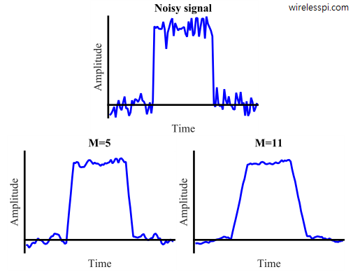
To see an example of noise reduction in time domain, consider a pulse in the figure below in which random noise is added. Observe that a longer filter performs a better smoothing action on the input signal. However, the longer length translates into wider edges during the transition.
We now explore how its magnitude response looks like.
Frequency Response
As a consequence of its flat impulse response, the frequency response of a moving average filter is the same as the frequency response of a rectangular pulse, i.e., a sinc signal.
Delving into details, the frequency response of this filter is the Discrete-Time Fourier Transform (DTFT) of $h[n]$ as follows.
\[
H\left(e^{j\omega}\right) = \sum_{n} h[n]e^{-j\omega n}
\]
Plugging in the impulse response, we get
\[
H\left(e^{j\omega}\right) = \sum_{n=0}^{M-1} \frac{1}{M}\cdot e^{-j\omega n} = \frac{1}{M}\sum_{n=0}^{M-1} \left(e^{-j\omega}\right)^n
\]
Using the familiar geometric series formula given by
\[
\sum \nolimits_{n=n_1}^{n_2} a^n = \frac{a^{n_1} – a^{n_2+1}}{1-a},
\]
we can write
\begin{equation}\label{equation-response}
\begin{aligned}
H\left(e^{j\omega}\right) &= \frac{1}{M}\frac{1 – e^{-j\omega M}}{1 – e^{-j\omega}} = \frac{1}{M}\frac{e^{-j\omega\frac{M}{2}} \left(e^{+j\omega\frac{M}{2}} – e^{-j\omega \frac{M}{2}} \right)}{e^{-j\frac{\omega}{2}}\left(e^{+j\frac{\omega}{2}} – e^{-j\frac{\omega}{2}} \right)} \\\\
&= e^{-j\omega\frac{M-1}{2}} \cdot \frac{1}{M}\frac{\sin \left(\omega M/2 \right)}{\sin \left( \omega/2\right)}
\end{aligned}
\end{equation}
where the relation $j2 \sin \theta = e^{+j\theta} – e^{-j\theta}$ is used in the last step. The first term above is the phase part which can be eliminated if the impulse response is centered around $n=0$. The frequency response is now expressed in a more common form by plugging in $\omega=2\pi f$ as
\begin{equation}\label{equation-moving-average-spectrum}
H\left(f\right) = \frac{1}{M}\frac{\sin \left(\pi M f\right)}{\sin \left( \pi f\right)}
\end{equation}
Here, $f$ is the discrete frequency defined as
\[
f = \frac{F}{f_s}
\]
where $F$ is the real frequency in Hz and $f_s$ is the sample rate. When $M$ is large, the numerator, $\sin(\pi fM)$, grows significantly with $M$ but the denominator stays the same. Therefore, the above magnitude response can be approximated as a sinc function.
\[
H\left(f\right) \approx \frac{\sin \left(\pi M f\right)}{\pi M f} = \text{sinc} (M f)
\]
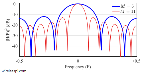
The magnitude response of such a filter is drawn in the figure below. It is far from the brickwall response of an ideal lowpass filter but the magnitude response still has a shape that passes low frequencies with some distortion and attenuates high frequencies to some extent.

Due to this insufficient suppression of sidelobes, it is probably the worst lowpass filter one can design. On the other hand, as described earlier, its simplicity of implementation makes it useful for many applications requiring high sample rates including wireless communication systems. In such conditions, a cascade of moving average filters is implemented in series such that each subsequent filter inflicts more suppression to higher frequencies of the input signal.
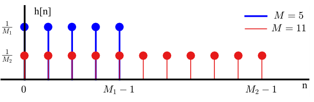
Due to the inverse relationship between time and frequency domains, a longer filter in time domain produces a narrower frequency response. This can be observed in the impulse and frequency response for filter lengths $M=5$ and $M=11$.
Zero Crossing Locations: The zeros in the spectrum occur at the frequencies where $\sin(\pi Mf) = 0$, which happens when
\[
\pi Mf = k\pi, \quad k = \pm 1, \pm 2, \pm 3, \dots
\]
Solving for $f$, we get:
\[
f = \frac{k}{M}, \quad k = \pm 1, \pm 2, \pm 3, \dots
\]
For the first zero crossing, $k = 1$ and we get
\[
f = \frac{1}{M}.
\]
In terms of Hertz, since the sampling frequency is $f_s$, the first zero crossing is at $f_s/M$. In general, a rectangular signal of width $M$ in one domain produces a sinc signal in the other domain with zero crossings at integer multiples of $1/M$.
Phase response: From Eq (1), we get
\begin{equation}\label{equation-phase-response}
\phi (\omega) = -\frac{M-1}{2}\omega
\end{equation}
which is similar to a linear equation $y=mx$. As described in the article on FIR filters, a moving average filter generates a delay of $(M-1)/2$ samples (for odd $M$) in the output signal as compared to an input signal. We see next the reason behind this delay.
Group Delay: Group delay represents how the phase of a system affects the timing of different frequency components as they pass through. It is mathematically defined as
\[
\tau_g(\omega) = -\frac{d\phi(\omega)}{d\omega}
\]
Now a phase shift at a specific frequency means that signal components at that frequency are delayed.
\[
\sin(\omega (t-\tau)) = \sin(\omega t + \phi),\qquad \text{where}\qquad \tau = -\frac{\phi}{\omega}
\]
Comparing with the last equation, the derivative of phase with respect to frequency tells how rapidly phase changes. Applying this to Eq (3), we get
\[
\tau_g(\omega) = \frac{M-1}{2}
\]
i.e., if the phase response is linear, all frequencies experience a constant delay at the output of the filter.