Design of a Discrete-Time Differentiator

Many signal processing algorithms require computation of the derivative of a signal in real-time. Some of the examples are timing recovery, carrier frequency synchronization, FM demodulation and demodulation of LoRa signals. An analog or digital filter that computes such a derivative is known as a differentiator.

Before we design such a discrete-time differentiating filter, let us review some of the fundamentals.

A Derivative

---

The following quote is attributed to Heraclitus, a Greek philosopher, from 535 BC.

This was brought into the realm of science by Newton and Leibniz. The purpose of science is not only to investigate how things are, but also to understand how they change with time (or another variable). While the former can translate a physical process into a mathematical formulation $f(x)$, the derivative helps us find out the latter. A derivative is thus defined as
\begin{equation}\label{equation-derivative-definition}
f'(x) = \lim _{h\rightarrow 0} \frac{f(x+h)\; – f(x)}{h}
\end{equation}

As $h$ approaches zero, it represents the slope $\tan \theta$ of the line tangent to $f(x)$ at a point. This is because in the triangle formed by $f(x)$ and $f(x+h)$, the above expression becomes the ratio of the hypotenuse $f(x+h)\; – f(x)$ and the base $h$.

The main challenge faced by a DSP engineer is how to bring this operation out of the theory and apply it to real world signals. For this purpose, we first need to know how an ideal derivative filter looks like.

A Continuous-Time Differentiator

---

In continuous-time systems, the derivative of a signal is determined by using an Operational Amplifier (op-amp) in which a capacitor acts on the input while the negative feedback is provided by a resistor. The circuit diagram for an ideal differentiator is illustrated below.

Due to the virtual ground, observe that the current flowing through the capacitor is given by $I=C \cdot dV_{in}/dt$, all of which passes through the resistor, i.e., $I=-V_{out}/R$. Equating these two expressions forms the basis of differentiation operation carried out by this op-amp.
\[
V_{out} = -RC \frac{dV_{in}}{dt}
\]

Our purpose is to design a discrete-time differentiator that is a Finite Impulse Response (FIR) filter. For this purpose, we need to know how an ideal derivative filter looks like.

The Ideal Derivative Filter

---

Consider a continuous-time signal $x(t)$ whose Fourier Transform is given by $X(\tilde \omega),$ where $\tilde \omega$ is the continuous frequency. The signal can then be expressed with the help of the inverse Fourier Transform.
\[
x(t) = \frac{1}{2\pi}\int _{-\infty}^{+\infty} X(\tilde \omega) e^{j\tilde \omega t}d\tilde \omega
\]

Differentiating both sides of the above equation, we get
\[
y(t) = \frac{dx(t)}{dt} = \frac{1}{2\pi}\int _{-\infty}^{+\infty} \Big[j\tilde \omega X(\tilde \omega) \Big]e^{j\tilde \omega t}d\tilde \omega
\]

The right side above is the inverse Fourier Transform of $Y(\tilde \omega)=j\tilde \omega X(\tilde \omega)$. In words, the derivative operation in time domain results in a product between $j\tilde \omega$ and $X(\tilde \omega)$ in frequency domain.
\[
Y(\tilde \omega) = j\tilde \omega X(\tilde \omega) = H(\tilde \omega)X(\tilde \omega)
\]

In conclusion, a filter that computes the derivative of a signal in time domain has a frequency response given by
\[
H(\tilde \omega) = j\tilde \omega
\]

In discrete domain, the frequency is normalized by the sample rate $F_s$, i.e., $\omega = \tilde \omega/F_s$ with the range betweeen $-\pi$ to $+\pi$. For a normalized sample rate $F_s=1$, the Discrete-Time Fourier Transform (DTFT) of an ideal derivative filter is given by

This frequency response of an ideal differentiator is shown in the figure below.

This will serve later as our guide in designing efficient discrete-time differentiators.

Simple Discrete-Time Differentiators

Let us start with the first difference filter.

First Difference

---

The simplest possible discrete-time differentiator merely emulates the continuous-time derivative in Eq (\ref{equation-derivative-definition}). Since the smallest unit of time in discrete domain is 1 sample, a first-difference filter is defined through the relation
\[
y_{FD}[n] = x[n] – x[n-1]
\]

From this expression, we can write the impulse response $h_{FD}[n]$ of a first-difference differentiator as
\begin{equation}\label{equation-first-difference-impulse-response}
h_{FD}[n] = \delta[n] – \delta[n-1] = \big\{1, -1\big\}
\end{equation}

where $\delta[n]$ is a unit impulse signal. The DTFT of the first difference filter is written as
\[
H_{FD}(\omega) = \sum _n \Big\{\delta[n] – \delta[n-1]\Big\}e^{-j\omega n} = 1 – e^{-j\omega}
\]

where $n=0$ and $n=1$ have been substituted in $e^{-j\omega n}$, respectively. In the right side expression, take $e^{-j\omega/2}$ as common and use Euler’s formula to get
\begin{equation}\label{equation-first-difference-frequency-response}
H_{FD}(\omega) = je^{-j\omega/2} \cdot 2\sin(\omega/2)
\end{equation}

Such a frequency response is plotted in the figure below along with the ideal response. At a first glance, it looks like the legs of a giant spider from The Hobbit or Harry Potter series.

There are two properties of a non-ideal differentiator we need to focus on.

1. Linear Range: Clearly, the range over which $H_{FD}(\omega)$ follows the ideal curve is quite limited, up to $\pi/4$ or $0.25\pi$. This implies that the input $x[n]$ to the first difference filter must have a bandwidth limited to $0.25\pi/2\pi$, or 12.5% of the sample rate $F_s$.
2. High Frequency Noise: The term $\sin(\omega/2)$ in the response $H_{FD}(\omega)$ of Eq (\ref{equation-first-difference-frequency-response}) dictates the half sine wave within the full $2\pi$ range, which resembles a high-pass filter. This implies that all the interference, harmonics and particularly noise in the higher spectral region will get passed on into the output signal $y[n]$ after the filtering operation. Therefore, it is desirable that a differentiator should suppress all the high frequency spectral components immediately after the departure of the filter response from the ideal straight line.

Central Difference

---

To solve this problem, the first idea is to take an average of two consecutive samples of the derivative signal since averaging reduces noise due to its lowpass filtering characteristic. This is known as a central difference filter.
\[
y_{CD}[n] = \frac{(x[n+1] – x[n]) + (x[n]) – x[n-1])}{2} = \frac{x[n+1]- x[n-1]}{2}
\]

Its impulse response can be written as
\begin{equation}\label{equation-central-difference-impulse-response}
h_{CD}[n] = \frac{1}{2}\left\{\delta[n+1] – \delta[n-1]\right\} = \frac{1}{2}\big\{1, 0, -1\big\}
\end{equation}

The frequency response $H_{CD}(\omega)$ can be derived in a similar manner as the first difference response $H_{FD}(\omega)$ that comes out to be
\begin{equation}\label{equation-central-difference-frequency-response}
H_{CD}(\omega) = j\cdot \sin(\omega)
\end{equation}

It is also drawn in the figure above along with the ideal and first different responses. Notice the following.

1. The linearity range of the central difference filter is around $0.18\pi$. This implies that the input $x[n]$ to the central difference filter must have a bandwidth limited to $0.18\pi/2\pi$, or 9% of the sample rate $F_s$. This characteristic is inferior as compared to the first difference filter and we are losing in terms of usable bandwidth of the derivative filter. This is a price we pay for the benefit described next.
2. The term $\sin(\omega)$ in the response $H_{CD}(\omega)$ of Eq (\ref{equation-central-difference-frequency-response}) dictates a full sine wave within the full $2\pi$ range. Looking at the figure above, it is clear that the central difference filter performs a better job in restraining the high frequency spectral components as compared to the first difference filter.

Lyons’ Differentiators

---

Rick Lyons has provided two contenders for simple differentiation with the following coefficients.
\begin{align*}
h_1[n] &= G_1\left\{-\frac{1}{16}, 0, 1, 0, -1, 0, \frac{1}{16}\right\} \\
h_2[n] &= G_2\left\{-\frac{3}{16}, \frac{31}{32}, 0, -\frac{31}{32}, \frac{3}{16}\right\}
\end{align*}

where $G_1$ and $G_2$ are their gains, respectively, to be discussed shortly. Notice that they look similar but $h_1[n]$ is a length-7 filter while $h_2[n]$ is a length-5 filter. The impulse responses of all these simple differentiators discussed so far are drawn in the figure below.

Observe that except the first difference whose length is 2 (an even number), all the other differentiators have an odd number of samples. This implies that their group delays are given by integer number of samples.
\[
\text{Group Delay} = \frac{N-1}{2}
\]

This value is 0.5 for first difference, 1 for central difference, 3 for $h_1[n]$ and 2 for $h_2[n]$. An integer number of samples is important for applications where the signals in two parallel branches need to be aligned for further processing (e.g., multiplication down the chain), e.g., FM demodulation.

The frequency responses of Lyons’ differentiators are plotted in the figure below. Also shown in the dashed curve are the first difference and central difference responses for a comparison.

Observe that the linear range of operation of Lyons’ 1st differentiator $H_1(\omega)$ extends to approximately $0.35\pi/2\pi$, or 17.5% of the sample rate $F_s$, which is almost twice as compared to the central difference differentiator. On the other hand, the same range for Lyons’ 2nd differentiator $H_2(\omega)$ is quite close to $0.5\pi/2\pi$, or 25% of the sample rate $F_s$. This is a significant improvement over the 1st filter.

5-Point Standard Derivative

---

Finally, there are other options available for constructing a simple differentiator. For example, instead of a 2-point derivative defined in Eq (\ref{equation-derivative-definition}) from which the first and central difference differentiators were derived, the definition of a 5-point standard derivative can be used to design a different filter, the coefficients of which are given by
\[
h_5[n] = G_5\left\{-1, 8, 0, -8, 1\right\}
\]

where $G_5$ will be derived next. The linear range of operation for $h[n]$ is around 15% of the sample rate $F_s$. An attractive feature of its implementation is the absence of multiplications, as the coefficients $\pm 1$ are simply additions while the coefficients $\pm 8$ can be implemented through an arithmetic left shift by 3 bits. This is an advantage of having coefficients that are integer powers of 2.

Differentiator Gain

---

A filter should not impart a gain to the input signal due to the limited precision available to represent each binary number. An ideal differentiator is a straight line $|H(\omega)| = \omega$ in frequency domain. Hence, its slope is 1 and this is what its gain represents too.

From the definition of Discrete-Time Fourier Transform (DTFT), we have
\[
\left.\frac{\partial H(e^{j\omega})}{\partial \omega}\right|_{\omega=0} = \frac{\partial}{\partial \omega} \sum_{n=-M}^{M} h(n)e^{-j \omega n}\bigg\vert_{\omega=0} = -j\sum_{n=-M}^{M}nh(n)
\]

Let us apply this to the differentiators explained above where a negative sign inverts the final result.

• First difference:
  \[
  0(1) + 1(-1) = -1, \qquad \Rightarrow \qquad G_{FD} = 1
  \]

• Central difference:
  \[
  (-1)1+ 0(0) + 1(-1) = -2, \qquad \Rightarrow \qquad G_{CD} = 2
  \]

• Lyons’ first filter:
  \[
  (-3)\left(\frac{-1}{16}\right) + (-1)1 + 1(-1) + 3\left(\frac{1}{16}\right), \qquad \Rightarrow \qquad G_{1} = 1.625
  \]

• Lyons’ second filter:
  \[
  (-2)\left(\frac{-3}{16}\right)+(-1)\left(\frac{31}{32}\right) + 1\left(\frac{-31}{32}\right) + 2\left(\frac{3}{16}\right), \qquad \Rightarrow \qquad G_{2} = 1.19
  \]

• 5-point standard filter:
  \[
  (-2)(-1)+(-1)8 + 0(0) + 1(-8) + 2(-1), \qquad \Rightarrow \qquad G_{5} = 12
  \]

Therefore, the differentiator coefficients are divided by that factor for proper normalization. Otherwise, the slope of their magnitude responses would be different than 1, the value required to follow the ideal response $|H(\omega)|=\omega$.

For differentiators derived through empirical or numerical techniques, the spectral response is plotted and the slope at zero is computed through numerical methods as well.

Wideband Differentiators

---

The simple differentiators we encountered above exhibit a response proportional to a sine function in frequency domain. The deviation of sine from a straight line is what limits their linear operating range. This is why these differentiators cannot be applied to signals with a wider frequency content. Wideband signals require a wideband differentiator.

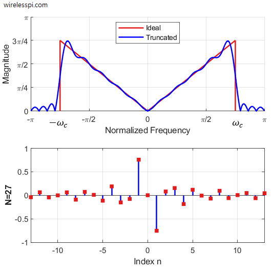
It is possible to design a wideband differentiator by building it from the fundamentals. Let us define a cutoff frequency $\omega_c$, before which the filter has a differentiating response and after which it should ideally pass no frequencies. Such a frequency response is plotted in the figure below.

The non-ideal spectrum labeled as ‘Truncated’ closely follows the ideal line but exhibits ripples across both sides of the cutoff frequency $\omega_c$ that is in the middle of a transition band. This is the Fourier Transform of the filter coefficients shown at the bottom of the same figure that form the impulse response of the differentiating filter. How did we come up with the filter taps? This can be accomplished in two ways.

• Take the inverse Fourier Transform of the desired response over the frequency range $-\omega_c \le \omega \le +\omega_c$.
  \[
  h[n] = \frac{1}{2\pi}\int _{-\omega_c}^{+\omega_c} j\omega e^{j\omega n}d\omega
  \]

  This integration by parts is an exercise in calculus because the frequency $\omega$ is a continuous variable. The reader is encouraged to derive $h[n]$ before moving on to the next easier route.

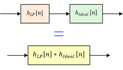
• Consider a lowpass filter within the range $-\omega_c \le \omega \le \omega_c$ with an impulse response $h_{LP}[n]$. The output of this lowpass filter is then passed through an ideal differentiator that yields the same output as from the differentiating filter in route 1 above. However, in this case, we have an option to combine these two filters in one by directly differentiating the impulse response $h_{LP}[n]$. This is shown in the figure below.

  

  Now the impulse response of a lowpass filter within the specified range $-\omega_c \le \omega \le \omega_c$ is a sinc sequence written in discrete time as
  \[
  h_{LP}[n] = \frac{\sin(\omega_c n)}{\pi n}
  \]

  Therefore, by taking the derivative of the above expression, we get the coefficients of our bandlimited differentiator.
  \begin{equation}\label{equation-wideband-differentiator-impulse-response}
  h[n] = \frac{\omega_c \cos(\omega_c n)}{\pi n} – \frac{\sin(\omega_c n)}{\pi n^2}
  \end{equation}

  which holds true for $-\infty < n < \infty$, except at $n \neq 0$ where $h[n]$ is zero. Treating the full-band differentiator as a special case, plug $\omega_c=\pi$ in the above expression that yields \begin{equation}\label{equation-full-band-differentiator-impulse-response} h[n] = \frac{\cos(\pi n)}{n} = \frac{(-1)^n}{n} \end{equation}

The rest of the story follows the usual signal processing plot (pun intended): truncation, large ripples as a consequence and windowing for smoothing them out.

The filter $h[n]$ has infinite coefficients which needs to be truncated for practical use.

• If we choose the filter length $N=3$, then there are only three coefficients, given by Eq (\ref{equation-full-band-differentiator-impulse-response}) as
  \[
  h_3[n] = \big\{1, 0, -1\big\}
  \]

  Except for the normalizing factor of $1/2$, this is exactly the central difference filter described in Eq (\ref{equation-central-difference-impulse-response}).

• The spectrum of the differentiator overlayed on the ideal response in the above figure exhibits large ripples due to its truncation at $N=27$ taps.

To overcome this behavior, a window such as as a Hamming window can be applied to the truncated sequence. For this purpose, we choose four different values of $N$, namely, $3$, $11$, $19$ and $27$. Using these values in Eq (\ref{equation-full-band-differentiator-impulse-response}) after applying a window generates the impulse responses shown in the figure below.

In this figure, the first central difference is scaled by $1/2$ to keep the filter gain equal for all values of $N$. A filter with a longer $N$ is expected to perform better. For this purpose, the resulting frequency responses are drawn in the figure below for the same values of $N$.

Observe from the above figure that the response gets better with an extended linear range as the filter length increases. Otherwise, there is not much difference between the filters. In other words, the advantage provided by longer filters is the ability to treat wideband signals effectively. Otherwise, for a low (normalized) frequency narrowband signal, a filter with a shorter length is preferable.

Another way of understanding this idea is that a low normalized frequency points to a high sample rate $F_s$. Viewing in time domain, a sufficiently oversampled signal should easily be differentiated by using only 2 to 4 samples, as these samples are close enough in this case. This is why a central difference filter is a good candidate for the derivative job as long as the input signal is at least 10 times oversampled.

On the other hand, there is an oscillation in the filters’ response around the ideal line due to the windowing effect. This creates excessive error within the passband of the differentiator. A solution to this problem is to apply some other window, say, a Blackman window, to the truncated differentiator impulse response which is drawn in the figure below for those values of $N$.

The frequency response with the Blackman window follows the desired response quite closely. However, due to its wide mainlobe, the linear frequency range becomes smaller than that of the Hamming window for the same $N$. This is the classic tradeoff we see in the windowing literature.

Which Differentiator to Use?

---

We have discussed several differentiators above and the question is which one of them should be employed in a signal processing application. It turns out that the best FIR filter design techniques, conventionally used for lowpass, highpass and bandpass applications, are of help here too.

• Parks-McClellan: The Parks-McClellan algorithm, also known as the Remez exchange algorithm, is a widely used method for designing digital filters with optimal frequency response. The filter is optimal in the sense that it minimizes the maximum error between the target frequency response and its actual frequency response. This is achieved by finding the best approximation through an iterative adjustment of the filter coefficients. The Parks-McClellan algorithm can also be employed to design discrete-time differentiators.

  For example, use the following command in Maltab for a full-band filter with length $N$.
  \[
  h_{PM} = \text{firpm(N-1,[0 0.5]*2,[0 pi],`differentiator’)}
  \]

  where the scaling factor of $2$ is included to overcome the flawed Matlab convention. My guess is that Matlab engineers made a mistake earlier of normalizing frequencies by $F_s/2$, while the actual normalization in DSP science is by $F_s$. And Matlab users have to follow this convention since then, just like the conventional current flowing from the positive to the negative direction.

• Least Squares: Least squares filter design is a technique used to find filters coefficients that minimize the sum of squared errors between the desired and actual responses. The process involves representing the desired frequency response as a set of discrete points and formulating a system of equations that is solved by using a least squares approach.

  For example, use the following command in Maltab for a full-band filter with length $N$.
  \[
  h_{LS} = \text{firls(N-1,[0 0.5]*2,[0 pi],`differentiator’)}
  \]

  where the scaling factor $2$ is again included for proper normalization as above.

The figure below plots the magnitude responses for both PM and LS algorithms (as well as the response errors) for a small value of $N=6$.

Observe that both responses are almost linear up to the full range. Moreover, the frequency response of the LS filter is better for the most part of this range. However, at the band edge (i.e., close to $\pm \pi$), it has a larger deviation than the PM from the ideal value (i.e., $\pi$). This is expected because the PM technique is designed to be optimal in minimizing the maximum error. This fact is more noticeable in the error response in the bottom subfigure.

One word of caution: The differentiator impulse response has odd symmetrical coefficients, proportional to $\cdots, +1, 0, -1, \cdots$. Therefore, for an odd-length $N$ filter, the frequency responses are zero at both $\omega=0$ and $\omega=\pi$. This follows from the Discerte-Time Fourier Transform (DTFT) definition. Assuming an odd $N=2M+1$, we have
\[
\begin{aligned}
H(0) &= \sum _{n=-M}^M h[n]e^{-j0 n} = 0 \\
H(\pi) &= \sum _{n=-M}^M h[n]e^{-j\pi n} = \sum _{n=-M}^M h[n] (-1)^n = 0
\end{aligned}
\]

where $e^{-j\pi n}=\cos \pi n = (-1)^n$ from Euler’s formula. As a consequence, odd-length differentiators, that exhibit a group delay in integer number of samples, cannot be used as full-band differentiators. This is important in applications where an integer group delay from the differentiating filter is required to align its output from another parallel stream for further processing. Efficient FM demodulation is one such example. Fortunately, partial-band differentiators can be designed and used with an inbuilt lowpass filtering feature.

Conclusion

---

In conclusion, discrete-time differentiation can be implemented through an FIR filter. There are several simple filters available designed through heuristic techniques but they work for highly oversampled signals due to their limited linear range of operation. On the other hand, filters designed through truncation and windowing are more suitable for wideband signals. However, they exhibit insufficient suppression of passband ripples and sidelobe levels. As in conventional filter design, differentiators created through optimal techniques like Parks-McClellan (PM) algorithm and Least Squares (LS) approach are more suitable for this task. For an inverse operation, see the article on discrete-time integrators.