Band Edge Filters for Carrier and Timing Synchronization

A Carrier Frequency Offset (CFO) arises due to a mismatch between Tx and Rx local oscillators as well as a phenomenon known as Doppler effect. In some other articles on this website, you will also find information on the Phase Locked Loop (PLL) in the context of carrier phase and timing synchronization.

There is another detailed post on the working of a Frequency Locked Loop (FLL) for carrier frequency synchronization which explains this concept with the help of a frequency error detector at symbol rate, i.e., after the acquisition of symbol timing offset. In many practical situations, the Carrier Frequency Offset (CFO) is large enough to render any timing synchronization unfeasible. Then, we have to resort to an FLL working at a multiple of symbol rate, i.e., at a rate of $L$ samples/symbol. Band edge filtering is one such example of a frequency error detector.

In the absence of timing and data, once a valid signal starts arriving, the timing offset can lie anywhere in the range $(0,T_M)$. The effect of an incorrect timing offset is such that the matched filter would remove a significant portion of the incoming signal energy, due to which we concentrate on a Rx signal sampled at a rate $F_S=1/T_S$. This sample rate is related to the symbol rate as $F_S = L/T_M$ where $L$ is the number of samples/symbol. The notations for the main parameters are the following.

• Sample time (inverse of sample rate): $T_S$
• Symbol time (inverse of symbol rate): $T_M$
• Number of samples/symbol: $L$
• Square-root Raised Cosine pulse shape: $p(nT_S)$
• Excess bandwidth: $\alpha$
• CFO: $F_\Delta$
• CFO estimate: $\hat F_\Delta$

The objective here is to determine a CFO estimate $\hat F_\Delta$ from the arriving signal. This feedback process is also known as Automatic Frequency Control (AFC).

Effect of CFO on Signal Energy

---

Assuming that the wireless channel has a flat frequency response, the energy out of the matched filter is maximum for a correct CFO estimate $\hat F_{\Delta}$ $=$ $F_{\Delta}$. Let us see why. The argument here suffices for a general understanding of the problem.

The Tx spectrum is shaped by a square-root Nyquist pulse $P[k]$ in frequency domain. In addition, the Rx signal is additionally shifted by an unknown CFO $F_{\Delta}$ by nature. This is depicted without any modulation through a blue solid line in the left column of the figure below.

Next, it is presented to the matched filter (another square-root Nyquist filter) centered at frequency $0$, which has a frequency response $P^*[k]$ shown as red dashed line in the figure above. The pulse shape is real and even, thus $P[k]$ as well as $P^*[k]$ are also real and even. In frequency domain, the output of a filter is its frequency response multiplied with that of the incoming signal. Therefore, only the overlapped region survives the filtering operation.

Now in the right column, the same figure shows the area under the magnitude squared of overlapped region which corresponds to the energy of the signal $z(nT_S)$ at the matched filter output. With this understanding, we take into account the following three cases.

1. For a large difference $\hat F_{\Delta}-F_{\Delta}$ as in the first case, the area under the overlapped region of the shaped signal and the matched filter is very small and consequently the energy $E_z$ of this output signal is low.
2. As the CFO estimate $\hat F_{\Delta}$ slides towards the second case of a reduced CFO difference, the overlapped area increases and so does the energy in $z(nT_S)$.
3. When $\hat F_{\Delta}$ approaches $F_{\Delta}$ in the third case, both the shaping filter and the matched filter completely overlap, the result is a perfect Nyquist spectrum and the signal energy attains its maximum value $P[k]^2$.

In summary, the output energy $\sum_n$ $|z(nT_S)|^2$ starts from zero for a very large difference between CFO and its estimate, increases towards a maximum value at $\hat F_{\Delta}=F_{\Delta}$ and then rolls down again in a symmetric fashion. In light of this discussion, the target of a non-timing-aided CFO compensation technique is to maximize this energy.

How to Maximize the Signal Energy

---

One route is to employ a feedback strategy suited to carrier acquisition in this setup. Instead of finding a closed-form expression for $\hat F_{\Delta}$, we form a frequency error detector proportional to $F_{\Delta}$ that drives an FLL maximizing $|z(nT_S)|^2$ in a recursive manner. Note the absence of summation here. It would have been there for a feedforward scheme but the strategy here is to compute an error signal for each feedback iteration of an FLL, just like we did before for a PLL.

After removing the summation, our goal is to maximize the energy with respect to the CFO estimate. Using the notation $\overset{\centerdot}{}$ for a derivative from here onwards, we can proceed as follows.

For a real signal, we could take the derivative of the target expression.
\begin{equation*}
\frac{d}{d \hat F_{\Delta}} |z(nT_S)|^2 = 2 z(nT_S) \cdot \overset{\centerdot}{z}(nT_S)
\end{equation*}

Can we carry on with the real signals? A shifted spectrum here dictates that complex signals need to be used. But don’t worry. We will keep the maths to a minimum. If you know about complex signals and what a conjugate operation means, then you can write
\begin{equation*}
|z(nT_S)|^2 = z(nT_S) \cdot z^*(nT_S)
\end{equation*}
In this case, the derivative is given by
\begin{align}
\frac{d}{d \hat F_{\Delta}} |z(nT_S)|^2 &= \frac{d}{d \hat F_{\Delta}}\left\{z(nT_S)\cdot z^*(nT_S) \right\}\nonumber\\
&= z(nT_S) \left\{\overset{\centerdot}{z}(nT_S)\right\}^* + \overset{\centerdot}{z}(nT_S) z^*(nT_S) \nonumber\\
&= z(nT_S) \left\{ \overset{\centerdot}{z}(nT_S)\right\}^* + \left(z(nT_S) \left\{ \overset{\centerdot}{z}(nT_S)\right\}^*\right)^*\nonumber\\
&= 2 \left\{z(nT_S) \cdot \left\{ \overset{\centerdot}{z}(nT_S)\right\}^*\right\}_I\label{eqFreqSyncMLFEDderivative}
\end{align}

where $I$ denotes the inphase component of the term within the brackets. The last equation follows from the fact that a complex signal added with its conjugate produces twice its inphase component.

To find the maximum of the curve, we equate the derivative to zero. On the other hand, the purpose of an FLL is to drive an error signal to zero as well. Combining these two facts, we can utilize this derivative as an error signal (neglecting an irrelevant factor of $2$).
\begin{align}\label{eqFreqSyncMLFED}
e_D[n] = \left\{z(nT_S)\cdot \left\{\overset{\centerdot}{z}(nT_S)\right\}^* \right\}_I
\end{align}

Such an error signal is commonly known as a maximum likelihood Frequency Error Detector (FED). Whilst the error signal is obtained, finding the derivative of a time-varying Rx signal after matched filtering in real-time is not a desirable signal processing operation. We want to convert the FED output into a more practical formation.

The Two Filters

---

Now there can be two ways to proceed from here.

1. Pass the matched filtered output $z(nT_S)$ through another filter $h(nT_S)$ that computes the derivative of its input in frequency domain. Here, the matched filter and the frequency domain derivative filter appear in series as shown in the figure below.
2. As far as the inphase component of $z(nT_S)\cdot (\overset{\centerdot}{z}(nT_S))^*$ is concerned, it makes sense to create a separate filter based on the pre-computed derivative of the matched filter with respect to frequency. It is usually known as a Frequency Matched Filter and denote its impulse response by $h_{FMF}(nT_S)$. To see why this approach works, consider the matched filter output through a differentiator (where $\tilde x(nT_S)$ is the matched filter input).
   \begin{align*}
   \overset{\centerdot}{z}(nT_S) &= z(nT_S) * h(nT_S) \\
   &= \Big\{\tilde x(nT_S) * p(-nT_S)\Big\} * h(nT_S)\\
   &= \tilde x(nT_S) * \underbrace{\Big\{p(-nT_S)*h(nT_S)\Big\}}_{h_{FMF}(nT_S)}
   \end{align*}

   Here, the two filters, namely the matched filter and the frequency matched filter, appear in parallel as shown in the figure below. The expression `The Two Filters’ is obviously taken from `The Two Towers’ in The Lord of the Rings by J. R. R. Tolkien. (For a maths purist, these two approaches are equal only with respect to inphase component of their product error signal that suffices for our purpose of extracting a frequency error signal.)

As an example, let us construct a continuous-time frequency matched filter for a square-root Nyquist pulse, say a Square-Root Raised Cosine (SRRC).

A Frequency Matched Filter

---

In the article on pulse shaping filter, we derived the frequency domain formula for the SRRC pulse (here acting as a matched filter) as
\begin{equation}\label{eqFreqSyncSRRCFreq}
H_{MF}(F) = \left\{ \begin{array}{l}
\sqrt{T_M} \hspace{2.2in} 0 \le |F| \le \frac{1-\alpha}{2T_M} \\[15pt]
\sqrt{T_M}\cos \left\{2\pi\cdot \frac{T_M}{4\alpha} \left( |F| – \frac{1-\alpha}{2T_M}\right)\right\} \hspace{0.3in} \frac{1-\alpha}{2T_M} \le |F| \le \frac{1+\alpha}{2T_M} \\[15pt]
0 \hspace{2.45in} |F| \ge \frac{1+\alpha}{2T_M}\\
\end{array} \right.
\end{equation}

The most important point to notice in the above equation is that the transition band of a Square-Root Raised Cosine pulse is a quarter cycle of a cosine with width $\alpha/T_M$ (this transition band is a half-cosine in a Raised Cosine filter). This can be seen as follows. From the equation, the inverse period of the cosine is $T_M/4\alpha$ and hence the period in frequency domain is $4 \alpha/T_M$. However, it exists in the region
\begin{equation}\label{eqFreqSyncTransitionBandWidth}
\frac{1+\alpha}{2T_M} – \frac{1-\alpha}{2T_M} = \frac{\alpha}{T_M}
\end{equation}

which shows that the transition band is a quarter cycle of a cosine.

To derive our frequency matched filter, we take the derivative of Eq \eqref{eqFreqSyncSRRCFreq} for three distinct regions of the spectrum, remembering that the cosine below is in frequency domain, not time domain and the derivative is with respect to frequency in a frequency matched filter. Thus, the derivative of an SRRC pulse in frequency domain, i.e., a frequency matched filter $H_{FMF}(F)$, is
\begin{equation}\label{eqFreqSyncSRRCFreqDerivative}
H_{FMF}(F) = \left\{ \begin{array}{l}
0 \hspace{2.3in} 0 \le |F| \le \frac{1-\alpha}{2T_M} \\[15pt]
\sqrt{T_M} \left(-2\pi \cdot \frac{T_M}{4\alpha}\right) \sin \left\{2\pi \cdot \frac{T_M}{4\alpha} \left(+ F – \frac{1-\alpha}{2T_M}\right)\right\} \\[7pt]
\hspace{2.05in} +\frac{1-\alpha}{2T_M} \le F \le +\frac{1+\alpha}{2T_M} \\[15pt]
\sqrt{T_M} \left(+2\pi \cdot \frac{T_M}{4\alpha}\right) \sin \left\{2\pi \cdot\frac{T_M}{4\alpha} \left( -F – \frac{1-\alpha}{2T_M}\right)\right\} \\[7pt]
\hspace{2.05in} -\frac{1+\alpha}{2T_M} \le F \le -\frac{1-\alpha}{2T_M} \\[15pt]
0 \hspace{2.58in} |F| \ge \frac{1+\alpha}{2T_M}\\
\end{array} \right.
\end{equation}

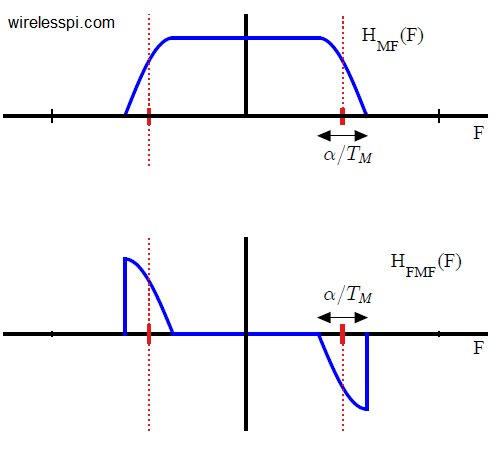
This frequency matched filter is drawn in the figure below for $\alpha$ $=$ $0.25$ corresponding to an SRRC pulse. Looking at the frequency response, it is easy to understand why the frequency matched filter is often called a band edge filter (other more practical band edge filters are also possible as we will see). From the figure, it is also clear that only the transition bandwidth contributes towards forming the frequency matched filter. For excess bandwidth $\alpha=0$, there would have been no frequency matched filter. In other words,

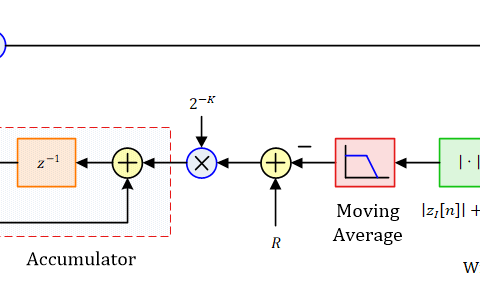
Observe that the frequency matched filter is indeed a quarter cycle of a negative sine wave in frequency domain. This can be more clearly visualized if you imagine $\alpha$ increasing towards $1$ in the figure above that will join the two band edges at the origin. This negative sine arises due to the transition band of the original matched filter being a quarter cycle of a cosine with width $\alpha/T_M$ where $T_M$ is one symbol time. The corresponding Frequency Locked Loop (FLL) is shown below.

The dynamics and behaviour of the FLL thus formulated are not much different than those of a PLL. Needless to say, its non-timing-aided and non-data-aided nature warrants long acquisition and settling times as compared to aided frequency synchronization procedures. Do remember on the other hand that catching up with a frequency offset is much quicker for an FLL than with a phase offset for a PLL.

Towards Practical Band Edge Filters

---

We can trace the following steps towards practical band edge filters.

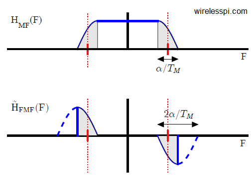
• As far as implementation is concerned, the actual coefficients of the discrete-time frequency matched filter $h_{FMF}(nT_S)$ are required. For this purpose, we first generate the discrete spectrum and then convert it into time domain coefficients through an inverse Discrete Fourier Transform (iDFT). However, we run into a problem. We said that the frequency matched filter has two parts: one at the edge of the positive band and the other at the edge of the negative band (which is why it is a kind of a band edge filter). Since the transition band of our matched filter contains a quarter cycle of a cosine, the frequency matched filter consists of a quarter cycle of a sine wave in both the positive and negative bands. This quarter cycle of the sine ends abruptly at the edges of the transition band and hence does not have a reasonably finite impulse response and depicts slowly decaying long tails.
• One approach to solve this problem is to continue the spectral shape past the discontinuity in the same trajectory such that the final spectral shape forms half a cycle of a sine wave. This relatively smooth transition towards zero imply a reduced time span and hence the time domain response of such a filter falls off quite rapidly as compared to the original frequency matched filter.

  

• Here is a new problem we face when we construct an error signal similar to Eq \eqref{eqFreqSyncMLFED} but with the derivative term replaced with modified frequency matched filter output: the error signal in time domain is formed by the product of the matched and modified frequency matched filter outputs. This product in time domain is a convolution in frequency domain between the spectrum of the matched filter output (which spans the full signal bandwidth) and that of the modified frequency matched filter output (which is limited in bandwidth). This convolution implies sliding one over the other and hence the resultant signal possesses the maximum amount of undesirable spectral components known as self-noise.

The main point is that the problem is not with the modified frequency matched filter anymore but with the matched filter that corrupts the resultant error signal by producing extra self-noise. Due to this reason, we consider implementing a set of filters with independent band edges.