The Discrete Fourier Transform (DFT)

Learned in some other articles on this website, the following three important concepts take us to the core of the Discrete Fourier Transform (DFT) idea.

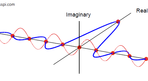
1. Regardless of the signal shape, most signals of practical interest can be considered as a sum of complex sinusoids oscillating at different frequencies.
2. A set of $N$ orthogonal complex sinusoids can be constructed within a span of $N$ time domain samples.
3. Each `tick’ or bin on the discrete frequency axis denotes the discrete frequency $k/N$ of such a complex sinusoid.

To understand how a set of sinusoids with $N$ discrete frequencies can sum up to a discrete-time signal of an arbitrary shape, we give an example of the $3$ dimensions of space, namely $x$, $y$ and $z$. Any point in space can be represented with a combination of just these $3$ basis components. We also studied different colours arising from the participation of just three basic colours: Red, Green and Blue.

The question is: if we are given $N$ samples of a discrete-time signal, how do we know the amplitude and phase contribution from each complex sinusoid in making up that signal? In the context of signal analysis, it turns out that the Discrete Fourier Transform} (DFT) is the tool that finds out the frequency domain amplitudes and phases of $N$ complex sinusoids present in a discrete-time signal of length $N$ samples.

Next, imagine a tool that takes a colour input and tells us how much of RGB contribution is there. Referring to RGB for example, it can inform us that
\begin{equation*}
\text{Yellow} =
\begin{cases}
100\% & \text{Red} \\
100\% & \text{Green} \\
0\% & \text{Blue}
\end{cases}
\end{equation*}
Or
\begin{equation*}
\text{Grey} =
\begin{cases}
50\% & \text{Red} \\
50\% & \text{Green} \\
50\% & \text{Blue}
\end{cases}
\end{equation*}

Similarly, the DFT finds in a discrete-time signal the amplitude and phase contributions $S[k]$ from each of the $N$ discrete-time complex sinusoids. These reference sinusoids given by $k/N$ are then called analysis frequencies. See how DFT decomposes the signal and outputs their respective contributions in Figure above.

Let us turn towards a formal definition of the DFT.

Definition

From the previous sections, let a discrete-time complex sinusoid be defined as $V[n]$.
\begin{equation*}
\begin{aligned}
V_I[n]\: &= \cos 2\pi\frac{k}{N}n\\
V_Q[n] &= \sin 2\pi\frac{k}{N}n
\end{aligned}
\end{equation*}
What we actually want to do is correlate (at lag $0$) a finite-length signal $s[n]$ with $N$ such complex sinusoids with frequencies $k/N$. From the article on correlation, it suffices to say that we multiply $s[n]$ with the complex sinusoid $V^*[n]$ sample-by-sample and take the sum. Then, the DFT $S[k]$ is given by
\begin{equation*}
S[k] = \sum \limits _{n=0} ^{N-1} s[n]V^*[n]
\end{equation*}
In terms of $s[n]$ with $I$ and $Q$ components $s_I[n]$ and $s_Q[n]$, the DFT $S[k]$ can be found through the application of multiplication rule of complex numbers.

for each $k$. In complex notation, this DFT is defined as
\begin{equation*}
S[k] = \sum \limits _{n=0} ^{N-1} s[n]\exp\left(-j2\pi\frac{k}{N}n\right)
\end{equation*}
In the above equation,

• $k$ is the index of DFT output in frequency domain, $k = -N/2$, $\cdots,-1,0,1$, $\cdots,N/2-1$
• $S[k]$ is $k^{th}$ DFT output component
• $S_I[k]$ and $S_Q[k]$ are $I$ and $Q$ components of the DFT $S[k]$
• $n$ is the time domain index of input samples, $n=0,1,\cdots,N-1$
• $s[n]$ is the sequence of input samples
• $N$ is the number of data samples in discrete time domain and number of bins in discrete frequency domain

Observe from the definition that each $S[k]$ output is computing the correlation at lag $0$ between an input signal and a complex sinusoid whose frequency is $-k$ complete cycles in an interval of $N$ samples (or $-k/N$ cycles per sample where a negative frequency implies clockwise rotation). Due to orthogonality, the correlation with all other $k’ \neq k$ is zero, popping out the contribution in the signal only from the complex sinusoid with frequency $-k/N$.

On the other hand, comparing with the phase rotation rule, we can observe that DFT operation is rotating a signal $s[n]$ clockwise.
\begin{align*}
I \cdot \cos (\cdot) + Q \cdot \sin (\cdot) \\
Q \cdot \cos (\cdot) – I \cdot \sin (\cdot)
\end{align*}
But what exactly does this mean?

The relation between a signal $s[n]$ and its Fourier Transform $S[k]$ is usually represented as
\begin{equation*}
s[n]\quad \rightarrow \quad S[k]
\end{equation*}

As a reminder, for a sample rate of $F_S=30$ kHz and $64$ point DFT, the fundamental frequency of the sinusoids is $F_S\cdot \pm 1/N = \pm 30,000/64 = \pm 468.75$ Hz represented by $k=\pm 1$. The other analysis frequencies are integer multiples of the fundamental frequency as

• $F_S\cdot \pm2/N = \pm937.5$ Hz represented by $k = \pm2$
• $F_S\cdot \pm3/N = \pm1406.3$ Hz represented by $k = \pm3$

and so on. Each frequency represents one complex sinusoid, or equivalently two real sinusoids.

Due to the periodicity of discrete frequency axis, DFT can also be defined for frequency bins $k=[0,N-1]$. However, the range $k = [-N/2,N/2-1]$ is more natural than $k=[0,N-1]$ since the former corresponds with our notion of a real sinusoid constituting one positive frequency and one negative frequency complex sinusoid. As an example, having two impulses in discrete frequency domain at $k = 5$ and $k = N-5$ does not seem to convey much information. However, viewing it as two impulses at $k = 5$ and $k = -5$ immediately makes one realize that the time domain signal is a real sinusoid with frequency $F_S\cdot 5/N$.

Inverse Discrete Fourier Transform (iDFT)

Just like DFT is used to convert a signal from time to frequency domain, Inverse Discrete Fourier Transform (iDFT) is used as an inverse process by converting a signal from frequency to time domain. iDFT is defined as

Notice that unlike DFT where the summation is over time index $n$, summation in iDFT is over frequency index $k$. Moreover, as opposed to DFT, the complex sinusoids here have a anticlockwise direction of rotation. In complex notation, this iDFT is defined as
\begin{equation*}
s[n] = \frac{1}{N}\sum \limits _{k=-N/2} ^{N/2-1} S[k]\exp\left(+j2\pi\frac{k}{N}n\right)
\end{equation*}
The iDFT is also a correlation like DFT as explained earlier. The amplitude scaling is $1/N$ to balance the factor $N$ that arises from the definition of orthogonality.

In words, iDFT equation is simpler to understand than the DFT equation since it is founded on our original premise that a signal can be represented as a sum of properly scaled complex sinusoids. From the definition of iDFT, observe that to reconstruct a signal $s[n]$, we have to sum $N$ complex sinusoids from $k=-N/2$ to $N/2-1$ after weighting them with DFT coefficients $S[k]$. This is the same concept where the time domain signal was made up of many sinusoids. The only difference is that in the case of continuous-time signals, the number of these sinusoids can go up to infinity.

DFT Periodicity

A natural consequence of DFT equation above is that $S[k]$ can be proved to be periodic with period $N$. Notice that the complex sinusoids making up the DFT output are periodic in $k$ because
\begin{equation*}
\begin{aligned}
\cos 2\pi\frac{k+N}{N}n = \cos \left\{ 2\pi \frac{k}{N} n + 2\pi n \right\} &= \cos 2\pi \frac{k}{N} n\\
\sin 2\pi\frac{k+N}{N}n = \sin \left\{ 2\pi \frac{k}{N} n + 2\pi n \right\} &= \sin 2\pi \frac{k}{N} n
\end{aligned}
\end{equation*}
Since the discrete frequency axis is itself periodic, i.e., the frequency $k/N$ and $(k+N)/N$ $=$ $k/N+1$ are the same, the DFT $S[k]$ is the same as $S[k+N]$. Thus,
\begin{align}
S[k + N] = S[k] \label{eqIntroductionDFTPeriodicityFreq}
\end{align}
It is not a surprising result that the DFT is a periodic signal in frequency domain due to the following reasoning. When we sample a continuous-time signal to obtain a discrete-time signal, infinite spectral replicas emerge that are spaced at integer multiples of the sample rate $F_S$. When we obtain the discrete frequency axis by sampling the baseband from $-0.5F_S$ to $+0.5F_S$ at $N$ equally spaced intervals, we are also implicitly sampling those spectral aliases and the DFT of a signal becomes periodic in frequency domain.

I personally consider the other approach more intuitive but it involves concepts like convolution and windowing which we have not covered yet and will encounter later. Since a common theme of this text is simplicity and periodic approach is simpler to follow, Eq \eqref{eqIntroductionDFTPeriodicityTime} will be our guide. All it says is the following:

“Although we know nothing about what happens with $s[n]$ outside the range $0$ to $N-1$, sampling the frequency axis at $N$ discrete points from $-N/2$ to $N/2-1$ creates replicas of $s[n]$ in time domain, just like sampling in time domain created replicas of its spectrum $S(F)$ in frequency domain.”

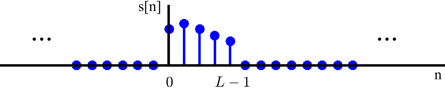
Figure below shows an aperiodic signal $s[n]$ and its periodic extension. As long as the DFT length $N$ is greater or equal to the signal length $L$, the DFT accurately represents the sampled frequency response of the input signal and there is no distortion. Nevertheless, for $N < L$, the DFT spectrum is no longer its actual sampled frequency domain representation and there will be aliasing in time domain. Obviously, common sense also dictates that taking DFT of a truncated input signal ($N < L$) should produce inaccurate results.

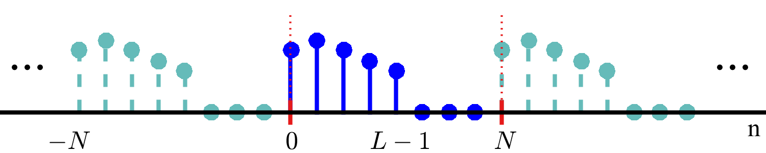
A major implication of this periodic extension is that sequence shifts for DFT purpose actually result in circular shifts. Assume $N = L$ in Figure above. Then, a right shift of $1$ will knock the last sample at position $n=N-1$ out of the observation window $[0,N-1]$ to the new position $n=N$. Moreover, it will bring the last sample from its previous extension at $n=-1$ inside the observation window to $n=0$. Conceptually, this is nothing but a circular shift within the window $[0,N-1]$. This DFT observation window is shown as red dotted lines within $0$ to $N-1$.

DFT Approximation of the Actual Spectrum

A natural question at this stage is: how well does the DFT — a sampled frequency function of a sampled time domain signal — approximates the underlying Fourier transform — a continuous frequency function of a continuous time domain signal? An initial guess is that it is not much accurate because the continuous Fourier transform is an integral from $-\infty$ to $\infty$ while the DFT is a finite sum.

The actual answer is that this approximation is quite well. However, there are two possible sources of error.

• [Truncation error] Clearly, any signal $s[n]$ that does not have a finite length must be truncated to accommodate finite length of the DFT.
• [Aliasing error] According to sampling theorem, the sample rate must be at least twice than the maximum frequency contained in $s[n]$. Aliasing can occur if the signal is not band-limited.

We discussed before that every real signal occupies an infinite amount of bandwidth, as a signal cannot be limited in both time and frequency domains. To avoid truncation errors, a signal must be time-limited which makes its spectrum unlimited causing aliasing errors. To avoid aliasing errors, a signal must be ideally band-limited with a sufficient sample rate, but such a signal cannot have finite duration causing truncation errors.

For many cases of practical interest, the amount of these errors is tolerable: with a reasonably band-limited signal that means having very small energy outside a certain frequency band, we can make the signal time-limited and sample it with an adequate sampling rate. That makes the DFT a great tool for analyzing real continuous-time signals.

Fast Fourier Transform (FFT)

A Fast Fourier Transform (FFT) is neither another type of Fourier transform, nor an approximation to the DFT. An FFT is just a faster method of computing the DFT of a signal by exploiting redundancy in DFT equations. In fact, it was FFT that made the Fourier analysis possible for majority of signal processing applications. For example, if FFT of a signal with length $N=10^6$ takes 1 second on a computing device, the DFT on the same platform will take approximately $28$ hours!

It is then no surprise that FFT is described as “the most important numerical algorithm of our lifetime”. Here, we will not derive the exact FFT formulation and instead will use a software routine to compute the FFT when required. In Matlab and Python, for example, the command fft($\cdot$) serves this purpose.

Concluding Remarks

For some examples of DFT in practice, you can read the article here. To test some of your own signals, you can check the code here.

Finally, instead of finding the spectrum that consists of all the frequencies in DFT, we are sometimes interested in the magnitude of one particular frequency in the signal. Computing a DFT becomes inefficient in that case. See the Goertzel algorithm as a great example of how to solve this problem.