One of the most common questions DSP beginners have is how to generate the signals (particularly, sinusoids) and view their spectrum. They have a rough idea what time domain and frequency domain are about but struggle to construct the first few lines of code that open the gates towards a deeper understanding of signals. For this reason, I produce below an Octave (or Matlab) code that you can simply copy and paste to view and modify the results.
- Keep in mind that the code has been written for an explanation purpose, not conciseness or optimization. As you progress towards developing a reasonably complicated DSP system, the coding aspect becomes more important.
- The code is verified on Octave version 4.2.2.
- Notice below that the main parameter to define first is the sample rate $F_S$. This then leads to simply following the theory to generate the signal and its spectrum.
Time Domain
For a theoretical background, you can read the article on the concept of frequency.
% Signal Generation

Fs = 10e3; Ts = 1/Fs; % sample rate and time
F1 = 1e3; T1 = 1/F1; % sinusoid frequency and period
nCycles = 4; % number of periods plotted

n = 0:1:nCycles*T1/Ts-1; % or t = 0:Ts:nCycles*T1-Ts;
A = 2;
phi = 0*pi/180;

st = A*cos(2*pi*F1/Fs*n + phi);
% or st = A*cos(2*pi*F1*t + phi) if you defined t above instead of n;


% Plotting

figure(1);

plot(n, st, 'LineWidth', 1, 'color', 'g')
axis([n(1) n(end) -A A])
set(gca,'XTick', 0:10:n(end),'YTick',-A:A);

hold on;

stem(n,st,'o','markerSize',7,'markerFaceColor','r',...
'markerEdgeColor','w','LineStyle','none')

xlabel('Time', 'FontSize', 12)
ylabel('Amplitude', 'FontSize', 12)
grid on
Here is the result of running this code.

Frequency Domain
For a theoretical background, see the Discrete Fourier Transform (DFT) and DFT examples. In frequency domain, the FFT size $N$ is the main parameter that should be carefully chosen.
nfft = length(n);
if mod(nfft,2) == 0
  k = -nfft/2:nfft/2-1; % discrete frequency index for even nfft
else
  k = -(nfft-1)/2:(nfft-1)/2; % discrete frequency index for odd nfft
end

% Discrete frequency Fd = k/nfft = F/Fs for example -0.5:1/nfft:0.5-1/nfft;

sf = fftshift(fft(st,nfft)); % fftshift for plot centered at Fd=0 instead of Fd=0.5

sfm = abs(sf); % magnitude response
sfmdB = 20*log10(sfm/max(sfm)); % division by max for normalizing the magnitude


% Plotting

figure(2);

plot(k, sfmdB, 'LineWidth', 1, 'color', 'g')
axis([-0.5 0.5 -60 0])
set(gca,'XTick', -0.5:0.25:0.5, 'YTick', -60:20:0)
hold on;

stem(k, sfmdB,'o','markerSize',7,'markerFaceColor','r',...
'markerEdgeColor','w','LineStyle','none')

xlabel('Frequency', 'FontSize', 12)
ylabel('Magnitude', 'FontSize', 12)
grid on
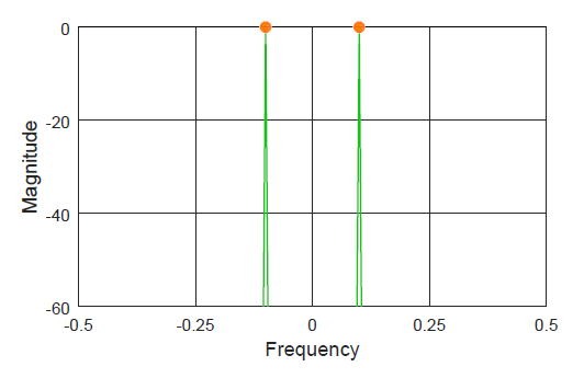
The result of running this code and plotting with Fd instead of k is as follows.

The spectrum of a sinusoid consists of two impulses, $+0.1$ and $-0.1$ in this case. These discrete frequency values appear from the ratio between the actual frequency and the sampling frequency.
\[ \frac{F1}{Fs} = \frac{1000}{10000} = 0.1 \] For a Python implementation of signal and spectrum generation, you can read about how to generate and detect Dual Tone Multi-Frequency (DTMF) signals.