In this article, we derive the spectrum of a complex sinusoid that acts as the basis for all spectra. In fact, the very definition of the Fourier Transform, whether continuous or discrete, comes from the perspective of a complex sinusoid. Therefore, exploring this derivation will be useful in everything else we learn about DSP.
Let us start with the continuous-time case.
A Continuous-Time Sinusoid
A continuous-time complex sinusoid with a frequency $f_b$ is defined as
\[
x(t) = e^{j2\pi f_b t} = \cos(2\pi f_bt) + j \sin(2\pi f_bt)
\]
This is known as Euler’s identity. Next, the Continuous Fourier Transform (CFT) is defined as
\[
X(f) = \int _{-\infty}^{+\infty} x(t) e^{-j2\pi f t}
\]
In all real scenarios, this complex sinusoid is limited within some duration, say of $T$ seconds. Therefore, we can write
\[
\begin{aligned}
X(f) &= \int _{-T/2}^{T/2} e^{j2\pi f_b t} e^{-j2\pi f t} \\
&= \int _{-T/2}^{T/2} e^{-j2\pi (f-f_b) t} = \frac{e^{-j2\pi (f-f_b)t}}{-j2\pi (f-f_b)} \Bigg|_{-T/2}^{T/2}
\end{aligned}
\]
because the integral of an exponential function is the exponential function itself, scaled by the constant being multiplied with the variable $t$. After simplification, we get
\[
X(f) = \frac{1}{j2\pi (f-f_b)} \left[e^{j2\pi (f-f_b)\frac{T}{2}} ~-~ e^{-j2\pi (f-f_b)\frac{T}{2}} \right]
\]
The expression in the brackets is $j2\sin(\cdot)$ from Euler’s identity.
\[
\sin \theta = \frac{e^{j\theta} – e^{-j\theta}}{2j}
\]
Consequently, we can write
\[
\begin{aligned}
X(f) &= \frac{\sin\left[2\pi (f-f_b)\frac{T}{2}\right]}{\pi (f-f_b)} = T\frac{\sin\left[\pi (f-f_b)T\right]}{\pi (f-f_b)T}\\
&= T\text{sinc}\left[\pi (f-f_b)T\right] \qquad \text{where}\qquad \text{sinc}(x) = \frac{\sin(x)}{x}
\end{aligned}
\]
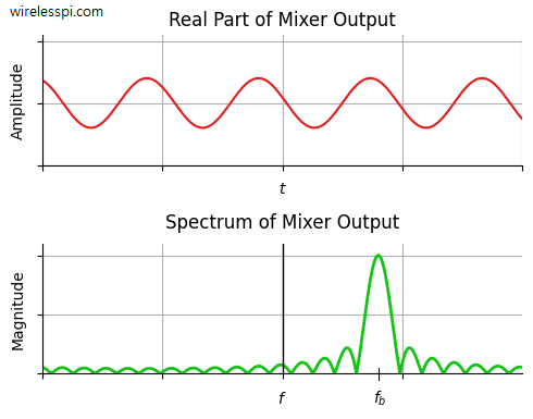
Since a sinc function has its peak at zero, we conclude that the Fourier Transform of a complex sinusoid is a sinc function shifted at frequency $f_b$. A limited duration continuous-time sinusoid and its spectrum are shown in the figure below, which is taken from the article on Frequency Modulated Continuous-Wave (FMCW) radar.

Let us explore how the same result can be intuitively derived.
Intuitive Reasoning
Intuitively, the same result can be reached by following the above figure which plots a sinusoid along with its spectrum.
- An infinitely long complex sinusoid with frequency $f_b$ in time domain has a spectrum that is an impulse at $f_b$.
- A rectangular signal in time domain is a sinc signal centered at DC in frequency domain.
- A limited duration waveform, like the sinusoid above, is similar to an infinite waveform multiplied with a rectangular signal.
- Multiplication in time domain is convolution in frequency domain.
- Convolution of the impulse at $f_b$ and the sinc signal centered at DC just puts the sinc signal at frequency $f_b$, as shown in the spectrum above.
We now turn our attention towards the discrete-time case.
A Discrete-Time Sinusoid
A discrete-time complex sinusoid with a frequency $k_o/N$ is defined as
\[
x[n] = e^{j2\pi \frac{k_o}{N}n} = \cos\left(2\pi \frac{k_o}{N}n\right) + j \sin\left(2\pi \frac{k_o}{N}n\right)
\]
To be consistent with the continuous-time case, the Discrete Fourier Transform (DFT) is defined for a length-$N=2L+1$ sequence as
\[
X[k] = \sum _{n=-L}^{L} x[n] e^{-j2\pi \frac{k}{N}n}
\]
where $k/N$ is the general discrete frequency. As opposed to other books and articles, I write the discrete frequency explicitly as $k/N$ so that one can immediately see the similarity behind $2\pi ft$ and $2\pi (k/N)n$ and recognize the discrete frequency, which loses its meaning when expressed as $2\pi kn/N$.
Now, applying the DFT definition,
\[
X[k] = \sum _{n=-L}^{L} e^{j2\pi \frac{k_o}{N}n} e^{-j2\pi \frac{k}{N}n} = \sum _{n=-L}^{L} e^{-j2\pi \frac{k-k_o}{N}n}
\]
The geometric series formula can be applied here.
\[
\sum _{n=N_1}^{N_2} a^n = \frac{a^{N_1} – a^{N_2+1}}{1-a}
\]
This leads us to the following expression.
\[
X[k] = \frac{e^{j2\pi \frac{k-k_o}{N}L} – e^{-j2\pi \frac{k-k_o}{N}(L+1)}}{1-e^{-j2\pi \frac{k-k_o}{N}}}
\]
Taking $e^{-j\pi\frac{k-k_o}{N}}$ common from both the numerator and the denominator, further simplification of this expression yields
\[
X[k] = \frac{e^{j2\pi \frac{k-k_o}{N}\left(L+\frac{1}{2}\right)} – e^{-j2\pi \frac{k-k_o}{N}\left(L+\frac{1}{2}\right)}}{e^{j\pi \frac{k-k_o}{N}}-e^{-j\pi \frac{k-k_o}{N}}} = \frac{\sin\left[ \pi \frac{k-k_o}{N}\left(2L+1\right)\right]}{\sin\left[\pi \frac{k-k_o}{N}\right]}
\]
This result — known as an aliased sinc function or a Dirichlet Kernel — is similar to the continuous-time case in that the numerator is $2\pi$ times half the temporal support. But it is different in the denominator where we have another $\sin(\cdot)$ function. For large $N$, the denominator approaches the sine argument itself (since $\sin\theta \approx \theta$ for small $\theta$) and becomes much smaller than the numerator. Therefore, it becomes a sinc function as well. So when $\pi k/N$ is small, we get
\[
X[k] \approx \frac{\sin\left[ \pi \frac{k-k_o}{N}\left(2L+1\right)\right]}{\pi \frac{k-k_o}{N}} = (2L+1)\text{sinc}\left[ \pi \frac{k-k_o}{N}\left(2L+1\right)\right]
\]
which corresponds to the continuous-time scenario derived above. In the limiting case, this sinc function reduces to a single impulse.
In relation to this derivation, you might also like the role of symmetry in Fourier Transform.