FMCW Radar Part 1 – Ranging

In his book Multirate Signal Processing, Fred Harris mentions a great problem solving technique:

"When faced with an unsolvable problem, change it into one you can solve, and solve that one instead."

We will see in this article how an FMCW radar is one of the most beautiful applications of this approach.

• The apparently logical method to measure the range of an object is through estimating the time delay of a reflected wave (on the order of a few nanoseconds) that is both expensive and less accurate. We can associate the range with the frequency of a sinusoid and measure that instead. This proves to be much simpler and accurate.
• There is another surprising way to apply this idea here that can only be understood after delving into the details. Therefore, it is mentioned in the concluding section.

Background

Radar (Radio Detection and Ranging) is an extension of human sensory perception. To understand this idea, consider the following two points.

• Imagine a bat in a dark night or inside a cave. It utilizes a remarkable method called echolocation to navigate and locate its prey. This involves emitting higher frequency ultrasound waves through their mouth or nose (the transmitter) that bounce off various objects which are then detected by its finely tuned ears (the receivers). This enables the bat to detect an insect prey as small as a mosquito!



• In principle, anyone can do the same to detect an object through sound signals but our ears and brain have a significantly coarser resolution (besides, who wants to spend all the time howling). Looking elsewhere (no pun intended), while vision is the most powerful sensor nature has given to us, our eyes can only act as passive radars and make use of the light signals already present in the environment.
  What we can practically do is design a machine that utilizes the same principle but in the electromagnetic spectrum outside the visible range (RF, for example). This machine is a radar that never complains about transmitting high-energy waves all day long and processing the received signals as they return.

We will discuss one particular kind of radar, Frequency Modulated Continuous-Wave (FMCW) radar, in this series. It is particularly useful in short range applications such as object detection in self-driving cars for collision avoidance, heartbeat monitoring, vibration measurement in residential and industrial products, drones ranging and intrusion detection. It is interesting to note that FMCW radar waveform bears similarities to Long Range (LoRa) physical layer.

Since FMCW radars are widely used in automotive applications, we take the example of autonomous vehicles for explaining the idea.

Next, we describe the radar principle through a formal approach.

The Radar Principle

A radar emits electromagnetic energy in one or more directions and searches for reflections from an object in the returning signal.

We describe the information extraction process in terms of both real and complex signals.

Range

Assume that the Tx signal is a sinusoidal Continuous-Wave (CW) given by
\[
x(t) = A \cos (2\pi ft)
\]

where $A$ is the amplitude and $f$ is the frequency. If all this energy disappears into an empty sky, there is no return signal. However, if there is an object within the illuminated area, a building wall for example, then the return signal is
\[
y(t) = A_r \cos \big[2\pi f(t-\tau_0)\big] = A_r \cos \big[2\pi ft + \phi\big]
\]

Here, $A_r$ is the amplitude of the (now very weak) echo signal and $\tau_0$ is the delay incurred during the return trip between the radar and the target. This parameter contains all the information about the target range $d_0$ in its phase, since we can write from the above expression:
\begin{equation}\label{equation-fmcw-delay}
\phi = -2\pi f\tau_0, \qquad \text{or} \qquad \tau_0 = -\frac{\phi}{2\pi f}
\end{equation}

From the above figure, $d_0$ is the distance between the Tx and the Rx which is doubled due to the wave traveling back and forth in its journey. From Newton’s laws of physics, the time delay $\tau_0$ is then equal to $2d_0/c$ if $c$ is the speed of the electromagnetic wave.
\[
\phi = -2\pi f \frac{2d_0}{c} = -4\pi \frac{d_0}{\lambda}
\]

where $\lambda$ is the operating wavelength of the radar. From here, the distance is estimated as

The negative sign has been removed because it arose from a delay and is immaterial with respect to the distance. As we shortly see, this technique is not useful for ranging since the sinusoidal wave is periodic with period $2\pi$. Therefore, the phase $\phi$ is unambiguous only within the range $-\pi$ to $+\pi$. For practical radio frequencies, this turns out to be only a few cm at most.

Next, we turn towards how to determine the velocity.

Velocity

Introduced in high-school physics as a frequency change in moving objects, the Doppler shift was explained in detail during the discussion on small-scale fading in wireless channels.

Imagine that the car in the above figure is driven at a constant velocity of $v$ m/s in the opposite direction. For all further times $t$, the electromagnetic wave that had to travel $d_0$ m now has to cover a distance of $d_0 + v t$.
\[
y(t) = A_r\cos \left[2\pi f \left(t-\frac{2d_0+ 2v t}{c}\right)\right] = A_r\cos \left[2\pi f \left\{\left(1- \frac{2v}{c}\right)t – \frac{2d_0}{c}\right\}\right]
\]

Clearly, the initial range is still the same as Eq (\ref{equation-fmcw-range}) while the Doppler shift $f_d$ is the change in frequency given by

This yields the velocity as

The wave arriving at angle of $\psi$ would have the Doppler shift scaled by $\cos \psi$. Since it is only the speed and not the range that can be determined, CW radars are mainly used in motion and speed sensing applications.

Receiver Block Diagram

The derivation for range above is quite simplistic. An actual CW radar sends an unmodulated wave and removes the carrier on the return path for extracting the desired signal, a block diagram for which is drawn in the figure below. The multiplier shown in Rx chain is known as a mixer and its output is of main concern to a radar designer.

If you are a DSP beginner, think of the mathematical expressions in the following terms. What happens when two sinusoids are multiplied with each other? The result is two sinusoids, one at a difference frequency and the other at summation frequency.
\[
2\cos\left[2\pi f (t-\tau_0)+\theta\right]\cdot \cos\left[2\pi f t+\theta\right] = \cos \left[ -2\pi f\tau_0\right] + \underbrace{\cos \left[2\pi \cdot 2f t -2\pi f \tau_0 +2\theta\right]}_{\text{Filtered out}}
\]

The summation frequency is lowpass filtered to yield the difference frequency term only. Next, we describe how to derive the same result through complex signals.

CW, Complex Sinusoid and IQ Processing

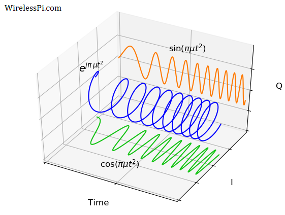
In practice, IQ signals are used whenever the phase is involved in a detection or estimation procedure. A Continuous Wave (CW) in IQ form is known as a complex sinusoid that is drawn in the figure below.

The expression for a complex sinusoid is given by $e^{j2\pi f t}$ where the instantaneous phase is a linear function of time.
\[
\phi = 2\pi ft
\]

The figure also demonstrates the Euler’s relation
\[
e^{j2\pi f t} = \cos (2\pi f t) + j\sin (2\pi f t)
\]

The real part $\cos (2\pi f t)$ can be seen as the projection of this complex sinusoid on the real plane (formed by time and $I$ axes). Moreover, the imaginary part $\sin (2\pi f t)$ can be seen as the projection of this complex sinusoid on the imaginary plane (formed by time and $Q$ axes).

We can now revisit the results for complex signals. In terms of complex signals, let the Tx signal be $e^{j(2\pi f t+\theta)}$ where we have included the phase $\theta$ ignored before. The received signal is its delayed version written as $e^{j[2\pi f (t-\tau_0)+\theta]}$. After a complex mixing process, we have
\[
y(t) = e^{j[2\pi f (t-\tau_0)+\theta]}\cdot e^{-j(2\pi f t+\theta)} = e^{-j2\pi f \tau_0}
\]

which has the same argument as the difference frequency above. Now let us explore why an unmodulated CW radar is not a very good idea.

Drawbacks of Unmodulated CW

In an ideal world, this simple CW gives us all the information we want. In practice, however, there are problems with this approach which limit the applications of CW radars.

• A CW radar cannot measure the range of a target. As described before, an unmodulated CW receives a phase $\phi$ that is unambiguous only within the range $-\pi$ to $+\pi$ because the mixer output is periodic with period $2\pi$. With no time or frequency markings, there is no way to differentiate between a, say, 100th cycle and 105th.
• The return signal amplitude $A_r$ is orders of magnitudes smaller than the Tx signal amplitude $A$. It is almost drowned by the Tx signal during the mixing and analog-to-digital conversion processes shown in the block diagram above. Separation between them needs to be achieved either through careful design to minimize leakage (monostatic) or physically separate antennas (bistatic).
• It is more difficult to combat the additive noise with a simple CW. In-band noise cannot be filtered out and adversely affects the estimation of phase and frequency. In fact, frequency estimation algorithms suffer from an SNR threshold effect: Below a certain SNR, the mean square error rapidly increases.
• In a multipath environment, the sum of multiple copies of such a signal exhibits the same frequency but a rotated phase given by their phasor addition. A modulated CW, as we will see later, can handle multiple reflections in a better way.
• It is very difficult to distinguish multiple targets around the radar since the returning waveforms from different objects overlap with each other with an effect similar to a multipath environment that distorts the phase and results in a loss of ranging information.
• The spectrum of a CW is a single narrow impulse. Therefore, it is more susceptible to interference from other transmissions.

As a consequence, we want an alternative technique and this is where modulation comes into the picture.

Pulse Compression

Let us explore what happens when a CW is modulated in time or frequency. The modulation acts as a marker against which the range can be determined, as we shortly see below. Moreover, the modulated signal bandwidth is no longer a single impulse. This expansion in frequency gives rise to a narrow signal in time domain which is advantageous for the radar. Think of an overlap among multiple return signals. Echos of such a narrow time domain signal can be clearly distinguished at the receiver.

Nevertheless, there are several practical obstacles from an RF circuit design perspective in generation and processing of a high-power short duration signal. The question is then how a short time duration can be achieved with minimal implementation complexity.

This idea gives rise to something known as a processing gain. Processing gain can be understood best by a Direct Sequence Spread Spectrum (DSSS) example. In this case, each data symbol is modulated with a spreading sequence that has a higher rate than the original data signal. This higher rate is known as processing gain or spreading factor. To recover the original data at the receiving end, the same sequence is employed and acts like a matched filter.

• Consider the box in the top subfigure below and notice how $-1$ in the echo and $-1$ in the matched filter are synced, as well as the remaining sequence. Therefore, a completely aligned copy of the same sequence at the receiver generates a much higher value during the point-by-point multiplication followed by a summation process (known as correlation). This is what acts as a marker for measurement purpose.
• Notice in the box shown in the bottom subfigure how $-1$ in the echo is multiplied with $+1$ in the matched filter and the output can be considered a random summation of $+1$s and $-1$s. Therefore, an unaligned sequence, even with the same values, generates a very small output as compared to the processing gain.

Common examples of DSSS systems include the Global Positioning System (GPS), IEEE 802.11b standard in WiFi networks and Code Division Multiple Access (CDMA) cellular systems.

Instead of a spreading sequence, an FMCW radar uses a chirp for a similar purpose, as shown in the figure below. A chirp is a signal with a linearly changing frequency. That is why this process is known as Linear Frequency Modulation (LFM).

Recall that a product of two sinusoids produces a difference and a sum frequency.
\[
2\cos\left(2\pi f_1 t\right)\cdot \cos\left(2\pi f_2 t\right) = \cos \left[ 2\pi (f_1-f_2)t\right] + \cos \left[2\pi (f_1+f_2) t\right]
\]

Summation over a long interval as performed in correlation thus produces low values for both terms above (since they have equal positive and negative halves), as shown in the bottom figure above.

On the other hand, a sinusoid multiplied with itself produces a DC gain in addition to a double frequency. Plugging $f_1=f_2=f$ in the above expression, we get
\[
2\cos^2(2\pi ft) = 1+\cos (2\pi \cdot 2f\cdot t)
\]

The sinusoid frequency is continuously changing in an FMCW wave. When correlated with itself in perfect alignment, similar frequencies line up together to generate a high peak, as shown in the top figure above. This is known as pulse compression that is achieved with the help of matched filtering.

Now let us find out how an FMCW waveform looks like.

FMCW Waveform

From a basic complex sinusoid that includes a linear instantaneous phase, we can move towards a basic chirp by extending it into a quadratic instantaneous phase, i.e., $e^{j\pi \mu t^2}$, where the reason behind the factor $\pi$ is explained soon. This signal is drawn in the figure below. Notice that instead of changing linearly over time, the phase is changing quadratically over time. This is why the signal seems to be compressed more and more to the right. Just like a frequency $f$ is the speed or rate of change of phase, a chirp rate $\mu$ is the acceleration of phase or rate of change of frequency.

From Euler’s relation, the real signal $\cos (\pi \mu t^2)$ can be seen as the projection of this complex sinusoid on the real plane (formed by time and $I$ axes). Moreover, the imaginary signal $\sin (\pi \mu t^2)$ can be seen as the projection of this complex sinusoid on the imaginary plane (formed by time and $Q$ axes).

It is common to draw this figure in 2 dimensions as shown below. The top subfigure is the same in-phase part of the complex chirp above for a chirp duration $T_C$.

• Here, it becomes clear why it can be seen as a CW modulated by a linearly changing frequency. The chirp spreads the spectrum and known as Chirp Spread Spectrum (CSS) in multiuser applications.
• Since the frequency is increasing, this waveform is known as an up-chirp. We will shortly see an example of a down-chirp too.

The spectrum of a chirp contains a wide band from the low initial frequencies to high final frequencies present in the signal. However, if you are familiar with FMCW radars, the bottom subfigure is what you would have seen before. To see where this comes from, let us write the general expression for the basic chirp, including the frequency and phase part.
\begin{equation}\label{equation-fcmw-basic-chirp}
x(t) = e^{j(\pi \mu t^2 + 2\pi f t+\theta)}
\end{equation}

The factor $\pi$ is actually $2\pi$ scaled by $1/2$. This is included to normalize the chirp rate taken as the slope of the instantaneous frequency (which is defined as the derivative of the argument).
\begin{equation}\label{equation-fmcw-nu1}
\nu(t)=\frac{1}{2\pi}\frac{d}{dt}\left(\pi \mu t^2 + 2\pi f t+\theta\right) = \mu t + f
\end{equation}

This is the relation drawn in the bottom subfigure above, where $f$ is the starting frequency (not the phase) shown as $0$ for simplicity (otherwise, the vertical axis should go from $f$ to $f+B$). Here, the chirp spans a bandwidth $B$ (called sweep bandwidth) over a time period $T_C$ (also known as sweep time). Hence, we can find the slope $\mu$ as
\begin{equation}\label{equation-fmcw-chirp-rate}
\mu = \frac{B}{T_C}
\end{equation}

The units of chirp rate $\mu$ should be Hz/second but it is common to measure it in terms of MHz/$\mu$s. In a typical transmission, several such chirps are transmitted in a sequence and the resultant FMCW waveform has a frequency vs time plot as shown below. Keep in mind that the actual IQ signal is still those spiraling chirps sent one after another.

For the sake of completeness, an up-chirp is not the only option an FMCW radar can utilize. A linearly decreasing frequency, known as a down-chirp is also possible, as drawn in the figure below. The actual signal and frequency vs time plot are shown on the left side.

In some situations, a combination of an up-chirp and a down-chirp proves more useful. This happens, e.g., when both static and moving objects need to be detected. Such a waveform, shown on the right side above, is called a triangular chirp.

We are now ready to see how an FMCW radar finds the range of a single target.

Range of a Single Target

An FMCW radar transmits a frequency modulated CW waveform in Eq (\ref{equation-fcmw-basic-chirp}). Assuming a single target at a distance of $d_0$ as before, the returning echo is a delayed version of the same signal. The delayed echo is drawn on the Tx time line in the figure below. Remembering that this is not the actual waveform, but a frequency vs time plot, a delay $\tau_0$ in the waveform also introduces a difference in frequency $f_b$, known as the beat frequency or Intermediate Frequency (IF). The expression beat frequency comes from the fact that it arises from the difference between the Tx and Rx chirps, as we shortly see in the DSP approach.

The range can be found by measuring the time delay $\tau_0$. However, the process of measuring small delays is much more complicated and inaccurate as compared to measuring the beat frequency through simple arithmetic operations.

There are three techniques to proceed from here.

Geometrical Approach

To find the relation between the time delay $\tau_0$ of the echo and the beat frequency $f_b$, consider the straight line in the above figure with slope $\mu$. Using the line equation $y=mx$, we can write
\[
f_b = \mu \tau_0
\]

Since $\tau_0=2d_0/c$ and $\mu=B/T_C$ from Eq (\ref{equation-fmcw-chirp-rate}), we have

Another way is to notice that the little triangle formed by $\tau_0$ and $f_b$ in the above figure is similar to the big triangle formed by the sweep time $T_C$ and sweep bandwidth $B$. Using the property of similar triangles that the ratios of their sides are equal, we get
\[
\frac{\tau_0}{T_C} = \frac{f_b}{B}, \qquad \text{or} \qquad \tau_0 = T_C\frac{f_b}{B}
\]

which is also equal to $2d_0/c$. This translates into a two-way distance expressed as
\[
d_0 = \frac{cT_C f_b}{2B}
\]

Now we see how the same result can be achieved in an intuitive manner.

Intuitive Approach

Since each mathematical expression is telling us a story, a commonsensical way to find the distance is the following.

• The chirp rate $\mu$ is the rate of change of frequency, or change in frequency per unit time.
• The chirp takes time $\tau_0$ to travel back and forth between the FMCW radar and the target.
• During this interval, the frequency changes by
  \[
  \begin{aligned}
  \text{Change in frequency} &= \frac{\text{Change in frequency}}{\text{Time}}\times \text{Time} \\
  f_b &= \mu \tau_0
  \end{aligned}
  \]

The rest of the derivation for $d_0$ stays the same. Next, we explore this issue through a DSP approach.

DSP Approach

The other method is the same as done before in the case of CW. The delayed waveform can be written as

\[
r(t) = e^{j[\pi \mu (t-\tau_0)^2 + 2\pi f (t-\tau_0)+\theta]}
\]

To keep the expressions simple, we are ignoring the amplitude factors here. Signal processing in radar is performed in discrete time but we can find out the major expressions in continuous time. A complex mixing process with the same waveform then yields

The only term containing $t$ above is the first one which determines the frequency of the output waveform: the beat frequency. Since the negative sign is immaterial with respect to the distance,
\[
2\pi f_b = 2\pi \mu \tau_0, \qquad \text{or} \qquad f_b = \mu \tau_0
\]

This can be simplified as
\[
\tau_0 = \frac{f_b}{\mu}
\]

We deduce the following.

The rest of the details are the same. Since $\tau_0=2d_0/c$ and $\mu=B/T_C$, we have

It turns out the same as derived through geometrical and intuitive approaches before.

In the expression for range $d_0$, all the parameters except the beat frequency $f_b$ are known because $c$ is the speed of the electromagnetic wave while $T_C$ and $B$ are system design parameters. Before we delve into that, however, we mention a point missed above.

But What About the Phase?

If you are a researcher, you would have immediately spotted something we missed in Eq (\ref{equation-fmcw-chirp-mixing-output}). The phase also contains some range information that could have been exploited to improve the estimate.
\[
\phi = \pi \mu \tau_0^2 ~-~ 2\pi f\tau_0
\]

While we only use beat frequency $f_b$ for the range, we see in Part 2 how this phase information is stitched together to find the velocity of a moving target.

Finding the Beat Frequency $f_b$

To find the beat frequency $f_b$ that completely determines the range from the Eq (\ref{equation-fmcw-single-target-range}) above, we need to discard the frequency vs time plot and refer to the actual waveform.

In reality, the delayed echo is mixed with a downchirp to generate the output, see Eq (\ref{equation-fmcw-chirp-mixing-output}) above.
\[
y(t) = e^{j2\pi f_b t +\phi}
\]

This waveform is nothing but a simple complex sinusoid! That is a CW with frequency $f_b$, the real part of which is plotted in the figure below along with its spectrum.

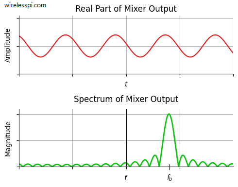
Why does the spectrum have a sinc shape? While DSP folks can look into the mathematical derivation for the spectrum of a sinusoid, the intuitive reasoning is as follows.

• An infinitely long complex sinusoid with frequency $f_b$ in time domain has a spectrum that is an impulse at $f_b$.
• A rectangular signal in time domain is a sinc signal at DC in frequency domain.
• A limited duration waveform, like the sinusoid above, is similar to an infinite waveform multiplied with a rectangular signal.
• Multiplication in time domain is convolution in frequency domain.
• Convolution of the impulse at $f_b$ and the sinc signal at DC just puts the sinc signal at frequency $f_b$, as shown in the spectrum above.

The problem is now reduced to finding the frequency of a sinusoid in noise. There are several techniques available to accurately estimate the frequency of a sinusoid in noise, see Chapter 6 of Wireless Communications from the Ground Up for a few examples.

Once $f_b$ is known, it can be plugged in Eq (\ref{equation-fmcw-single-target-range}) to determine the range. And this frequency is not limited within a $2\pi$ span like the phase!

A word of caution: It is easy to overlook the phase part in such calculations but it must be included for proper analysis, particularly in joint communications and sensing applications.

Range FFT

Imagine what happens when there are multiple targets present in the environment. For example, an autonomous vehicle has to determine its distances from all things around, as well as velocities of the moving objects. This includes other vehicles, buildings, lamp posts, pedestrians, and the likes.

Let us consider the case of stationary targets first. Moving targets will be described in Part 2.

Cumulative Signal

In this scenario, instead of receiving a single echo, the radar receives multiple echos overlapped with each other to form the cumulative signal. One such example is drawn below for 3 targets. The echos are arriving after time delays $\tau_0$, $\tau_1$ and $\tau_2$ while the beat frequencies generated after mixing are denoted by $f_{bo}$, $f_{b1}$ and $f_{b2}$, respectively. The higher the delay, the larger the beat frequency.

It is easy to think from the bottom subfigure above that the cumulative signal is a sum of three constants and hence a constant signal. But remember that this is a frequency vs time plot. The actual signal is formed by the reflections from 3 targets that are essentially 3 chirps with different parameters. This cumulative signal is plotted in the figure below. After chirp demodulation, it is straightforward to see that the output signal is a sum of 3 sinusoids, similar to Eq(\ref{equation-fmcw-chirp-mixing-output}).

This mixer output or IF signal can be written as
\[
y(t) = e^{j(2\pi f_{bo}t+\phi_o)} + e^{j(2\pi f_{b1}t+\phi_1)} + e^{j(2\pi f_{b2}t+\phi_2)}
\]

Due to multiple reflecting echos, the algorithm searching for the frequency of a sinusoid in noise cannot be employed. Instead, what we can do is to locate the peaks in the spectrum of the return signal above a certain threshold. How do we compute the signal spectrum?

Finding the Beat Frequencies $f_b$

Even DSP beginners have heard about the Fast Fourier Transform (FFT) algorithm, known as the algorithm of the 20th century due to its huge impact on science and technology. An FFT is nothing but an efficient implementation of Discrete Fourier Transform (DFT) defined for a length-$N$ sequence as
\[
Y[k] = \sum_{n=0}^{N-1} y[n]e^{-j2\pi \frac{k}{N}n}
\]

The above mathematical expression can be described in a nutshell as follows.

• Remember that frequency is defined as the rate of change of phase (sample-by-sample here).
• If $y[n]$ contains a component of frequency $+k/N$, sample-by-sample de-rotation by a complex sinusoid of the same frequency but opposite direction (i.e., $−k/N$) results in an output as a single number due to the corresponding phase canceling out at each step.
• That single number is naturally the amplitude of the complex sinusoid with frequency $k/N$, an indicator of how much that sinusoid contributes to the construction of $y[n]$.

The cumulative signal and the FFT output for reflections from 3 targets after the mixer is plotted below.

The whole FFT process eventually tries to find the participation of every such complex sinusoid in construction of the examined signal. And finding the contribution from sinusoids of different frequencies above a certain threshold is exactly what we want, see the figure above.

This gives us the beat frequencies of all three echos, and hence the target ranges by extension, see Eq (\ref{equation-fmcw-single-target-range}).

The whole ranging procedure can now be summarized in one figure as shown below. The frequency domain is indicated by a range axis due their interchangeability.

The reason FFT vectors are stacked in a vertical column instead of a horizontal sequence will become clear in Part 2 when we explore how an FMCW radar estimates the velocities of moving targets as well. Finally, a suitable window is applied to the IF signal samples before taking the FFT to minimize the DFT leakage.

Conclusion

In conclusion, an FMCW radar is one of the most beautiful examples of a real DSP application. As Fred Harris says: "When faced with an unsolvable problem, change it into one you can solve, and solve that one instead." There are two ways in which this principle can be applied here.

1. Measure the Frequency, Not the Time

While measuring the time delays on the order of a few nanoseconds is difficult, estimating the range of an object through beat frequency becomes a straightforward task. This beat frequency $f_b$ arises from a cross term during the mixing process between Tx and Rx chirps because $\mu \tau_0$ is the change in frequency per unit time multiplied with time, and hence similar to Doppler frequency.

In a real scenario, there are multiple objects in the surroundings and the reflected echos prove even more troublesome by overlapping with each other at the Rx. Instead, taking an FFT of the mixer output easily reveals their ranges through detection of peak frequencies.

2. Move the Signal if the Target Does Not

Looking back, a CW radar cannot measure the range of a stationary object but can estimate the velocity of a moving target. An intelligent person should flip this idea on its head. We can move the frequency by introducing a chirp (i.e., a linearly changing frequency) which — upon reflection — reveals the range of a stationary target!

It can be applied to our personal and professional interactions too. Rather than expecting the world to behave in a certain way, it is often easier to change something on our part that ultimately achieves the same objective.