LoRa PHY (Long-Range Physical Layer) is a very exciting communication technique based on Chirp Spread Spectrum (CSS) modulation mixed with Frequency Shift Keying (FSK). It is a proprietary physical layer methodology patented by Semtech. On the other hand, LoRaWAN is a Low Power Wide Area Network (LPWAN) protocol that is built on top of LoRa PHY. Some of the benefits of LoRa are
- resistance to multipath fading and Doppler effect,
- robustness against narrowband interference and jamming,
- low RF power consumption owing to the constant envelope signal,
- computationally simple from signal processing perspective,
- long-range transmission and reception, and
- inherent ranging capability due to linear frequency modulation.
This is why it has been popular as a physical layer in implementations of Internet of Things (IoT) systems that consist of battery-powered devices with low data rate connectivity over a long range. The use cases are as diverse as environmental monitoring, smart grids, agriculture efficiency, home and building automation, industrial control, disaster prevention and object localization.
The signals involved in this tutorial are mostly complex. For a reader who is just starting with DSP and wireless communications, I have two recommendations about the fundamentals.
- Learn about the origin of complex numbers and signals.
- Delve into why I/Q signals are used in signal processing applications in general and wireless communications in particular. This is also useful if you want to see the underlying sinusoidal signals in the PSK description below that focuses only on the instantaneous phase.
The starting point to learn about LoRa PHY is the simple phase modulation. This will help us cover the ideas behind LoRa PHY by a simple extension from phase to frequency.
Phase Shift Keying (PSK)
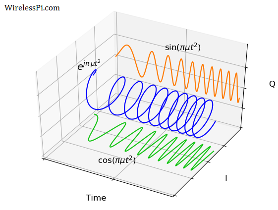
The most fundamental of all signals is a complex sinusoid given by
\[
x(t) = e^{j2\pi f t}
\]
This signal is drawn in the figure below.

The figure also demonstrates the Euler’s relation
\[
e^{j2\pi f t} = \cos (2\pi f t) + j\sin (2\pi f t)
\]
The real part $\cos (2\pi f t)$ can be seen as the projection of this complex sinusoid on the real plane (formed by time and $I$ axes). Moreover, the imaginary part $\sin (2\pi f t)$ can be seen as the projection of this complex sinusoid on the imaginary plane (formed by time and $Q$ axes).
Instantaneous Phase
The general expression for the complex sinusoid, ignoring the amplitude, is written as
\begin{equation}\label{equation-basic-complex-sinusoid}
x(t) = e^{j(2\pi f t+\theta)}
\end{equation}
The instantaneous phase is defined as the argument of this signal.
\[
\phi(t) = 2\pi f t + \theta
\]
Observe that there are two different parameters in the instantaneous phase that can be altered to transmit information.
- Phase $\theta$
- Frequency $\omega=2\pi f$
Modulation
Utilizing only the phase part, data can be sent through a set of $M$ phases $\theta_m$ where $m=0,1,\cdots,M-1$. For $M=4$, four different signals can be used to transmit two bits over a channel due to the relation $\log_2 4=2$. From Eq (\ref{equation-basic-complex-sinusoid}), we can write
\begin{equation}\label{equation-phase-modulation}
x(t) = e^{j(2\pi f t+\theta_m)}
\end{equation}
The instantaneous phase is
\[
\phi_m(t)=2\pi f t + \theta_m, \qquad m=0,1,\cdots,M-1, \quad\text{or}\quad m=-\frac{M}{2}, \cdots, \frac{M}{2}-1
\]
Take $M=4$ as an example. Within the possible range of $2\pi$, four such phases are multiples of
\[
\theta_1=\frac{2\pi}{M}=\frac{2\pi}{4}=\frac{\pi}{2} \qquad \qquad \text{and}\qquad\qquad \theta_m=m \theta_1
\]
where $m=-2, -1, 0$ and $+1$. An assignment from phase to bits can be in the form
\[
\begin{aligned}
\theta_{-2} = -2 \theta_1=-\pi \qquad &\rightarrow \qquad 00 \\
\theta_{-1} = -1 \theta_1=-\frac{\pi}{2} \qquad &\rightarrow \qquad 01 \\
\theta_0 = 0\cdot \theta_1=0 \qquad &\rightarrow \qquad 10 \\
\theta_{+1} = +1 \theta_1=+\frac{\pi}{2} \qquad &\rightarrow \qquad 11
\end{aligned}
\]
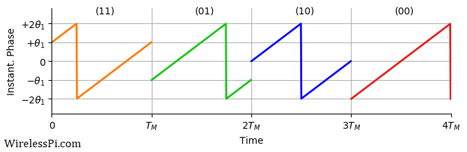
The four possible instantaneous phases $2\pi f t+\theta_m$ are drawn in the figure below. Observe the following.

- Since $\theta_1=\frac{2\pi}{4}=\frac{\pi}{2}$, the range can easily be verified as $-2\theta_1=-\pi$ to $+2\theta_1=+\pi$.
- The transmission rate is the inverse of one period $T_M$ that is known as a symbol time. It is the time period in which one of all possible modulation symbols are sent. Notice in the above figure how the instantaneous phase is wrapped at multiples of $\frac{1}{M}=\frac{1}{4}$ of the symbol time $T_M$ for each $m$.
- An example signal carrying the bit sequence 11 01 10 00 is drawn in the figure below.
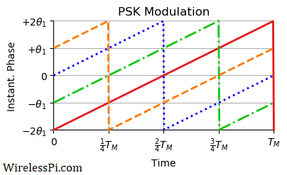
- From a signal construction perspective, these instantaneous phases are simply circular shifts (by symbol number $m$) of one basic signal $2\pi f t + \theta_0$ as shown in the figure below where the above four signals are drawn on top of each other.


Demodulation
On the receiver side, the complex sinusoid part of the signal is removed as it carries no information. What is left is the modulation phase. From Eq (\ref{equation-phase-modulation}),
\[
e^{j(2\pi f t + \theta_m)}\cdot e^{-j2\pi f t} = e^{j \theta_m}
\]
The argument of the above complex number reveals the data symbol at time $m$ that can then be translated into corresponding bits.
\[
\hat \theta_m = \measuredangle e^{j\theta_m}
\]
For ease of exposition, this downconversion is described as a theoretical process as a product with $e^{-j2\pi f t}$. In reality, the phase information is reflected in how the actual sinusoid starts and it is difficult to measure. See I/Q signals 101 to find out the actual phase to amplitude conversion process, the real reason behind the widespread use of I/Q signals.
Furthermore, there is a significant amount of details missing from the above description and implementing a real PSK receiver is not that straightforward a task. At the transmit side after the generation of modulation symbols, we have to do upsampling, pulse shaping to control the spectrum and upconversion of the signal to a suitable frequency. At the receive side, we have to downconvert the high frequency signal, remove the carrier frequency offset between the Tx and Rx oscillators, carry out matched filtering to maximize the Signal to Noise Ratio (SNR), acquire timing and phase synchronization and equalize the signal to mitigate the multipath channel effects, see Wireless Communications from the Ground Up – An SDR Perspective as a reference.
Now we turn from instantaneous phase to instantaneous frequency that extends the idea from PSK to FS-CSS in a straightforward manner.
Frequency Shift – Chirp Spread Spectrum (FS-CSS)
From a basic complex sinusoid that includes a linear instantaneous phase, we can move towards a basic chirp by extending it into a quadratic instantaneous phase.
\[
x(t) = e^{j\pi \mu t^2}
\]
where the reason behind the factor $\pi$ is explained soon. This signal is drawn in the figure below. Notice that instead of changing linearly over time, the phase is changing quadratically over time. This is why the signal seems to be compressed more and more to the right.

From Euler’s relation, the real signal $\cos (\pi \mu t^2)$ can be seen as the projection of this complex sinusoid on the real plane (formed by time and $I$ axes). Moreover, the imaginary signal $\sin (\pi \mu t^2)$ can be seen as the projection of this complex sinusoid on the imaginary plane (formed by time and $Q$ axes).
Instantaneous Frequency
The general expression for the basic chirp, ignoring the amplitude, is written as
\begin{equation}\label{equation-basic-chirp}
x(t) = e^{j(\pi \mu t^2 + 2\pi f t+\theta)}
\end{equation}
The factor $\pi$ is actually $2\pi$ scaled by $1/2$. This is included to normalize the chirp rate as the slope of the instantaneous frequency (which is defined as the derivative of the argument).
\begin{equation}\label{equation-nu1}
\nu(t)=\frac{1}{2\pi}\frac{d}{dt}\left(\pi \mu t^2 + 2\pi f t+\theta\right) = \mu t + f
\end{equation}
Observe that there are three different parameters in the instantaneous phase that can be altered to transmit information.
- Phase $\theta$
- Frequency $\omega=2\pi f$
- Chirp rate $\mu$
You can also read about an example of a Frequency Modulated Continuous-Wave (FMCW) radar using a similar techinque.
Modulation
Utilizing only the frequency part (if you are thinking about utilizing all the parameters, namely the amplitude, $\mu$, $f$ and $\theta$, for encoding information, you will have a high data-rate but a very complex modem that will be ill-suited from both design and application perspectives), data can be sent through a set of $M$ frequencies $f_m$ where $m=0,1,\cdots,M-1$. For $M=4$, four different signals can be used to transmit two bits over a channel due to the relation $\log_2 4=2$. From Eq (\ref{equation-basic-chirp}), we can write
\begin{equation}\label{equation-frequency-modulation}
x(t) = e^{j(\pi \mu t^2 + 2\pi f_m t+\theta)}
\end{equation}
From Eq (\ref{equation-nu1}), the instantaneous frequency as the derivative of the instantaneous phase is given by
\[
\nu_m(t)=\mu t + f_m, \qquad m=0,1,\cdots,M-1, \qquad\text{or}\qquad m=-\frac{M}{2},\cdots, \frac{M}{2}-1
\]
Take $M=4$ as an example. Within the possible range of bandwidth $B$, four such frequencies are multiples of
\begin{equation}\label{equation-mf1}
f_1=\frac{B}{M}=\frac{B}{4} \quad\text{and}\quad f_m = m f_1
\end{equation}
where $m=-2, -1, 0$ and $+1$. An assignment from frequency to bits can be in the form
\[
\begin{aligned}
f_{-2} = -2 f_1=-\frac{B}{2} \qquad &\rightarrow \qquad 00 \\
f_{-1} = -1 f_1=-\frac{B}{4} \qquad &\rightarrow \qquad 01 \\
f_0 = 0 \cdot f_1=0 \qquad &\rightarrow \qquad 10 \\
f_{+1} = +1 f_1=+\frac{B}{4} \qquad &\rightarrow \qquad 11
\end{aligned}
\]
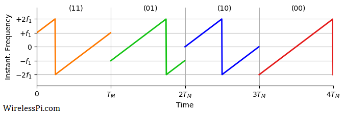
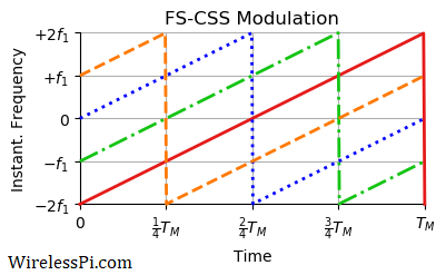
The four possible instantaneous frequencies $\mu t+f_m$ are drawn in the figure below. By comparing with the corresponding PSK figure, it becomes clear why these initial $M$ frequencies are also known as "chirp-phases". Looking at the y-axis, we also notice the similarity with Frequency Shift Keying (FSK) modulation. Observe the following.

- In terms of cycles/second or Hz, the frequency range can easily be verified as $-2f_1=-\frac{B}{2}$ to $+2f_1=+\frac{B}{2}$. In essence, this modulation is about linearly sweeping the signal frequency within a defined bandwidth. Many authors include a factor of $-B/2$ with modulation frequencies because they define the symbols for $m=0,1,\cdots,M-1$ as opposed to balancing them around zero as $m=-\frac{M}{2}\cdots,\frac{M}{2}-1$.
- Again, the transmission rate is the inverse of one period $T_M$ (the symbol time). It is the time period in which one out of all possible modulation symbols are sent. Notice in the above figure how the instantaneous frequency is wrapped at multiples of $\frac{1}{M}=\frac{1}{4}$ of the symbol time $T_M$ for each $m$.
- An example signal carrying the bit sequence 11 01 10 00 is drawn in the figure below.
- From a signal construction perspective, these instantaneous frequencies are simply circular shifts (by symbol number $m$) of one basic signal $\mu t + f_0$ as shown in the figure below where the above four signals are drawn on top of each other. This helps in constructing the symbols in hardware through efficient circular shifts.


Demodulation
On the receiver side, the raw chirp part of the signal is removed as it carries no information. What is left is the modulation frequency and an extra phase. From Eq (\ref{equation-frequency-modulation}),
\begin{equation}\label{equation-downconverted-chirp}
e^{j\left(\pi \mu t^2 + 2\pi f_m t+\theta\right)}\cdot e^{-j\pi \mu t^2} = e^{j (2\pi f_m t + \theta)}
\end{equation}
The slope in the above argument reveals the data symbol at time $m$ that can then be translated into corresponding bits. In most cases, the simplicity of devices implementing LoRa protocol necessitates removal of phase $\theta$ without estimation, e.g., by employing conjugate multiplication and absolute values. This is a non-coherent approach as explained in detail below. On the other hand, a coherent receiver estimates and removes this phase directly or through a Phase Locked Loop (PLL) in a typical performance-complexity tradeoff.
Finding this slope $f_m$ is exactly the same problem as finding a complex sinusoid in noise with an arbitrary phase. There is a long history of solutions in DSP and wireless communications to estimate the frequency of a sinusoid in noise. We will describe only one simple algorithm for accomplishing this task in LoRa demodulation.
Next, we turn our attention towards how FS-CSS is used in LoRa PHY.
LoRa PHY Signal
The aim of LoRa PHY is to achieve excellent link budget at low power for long-range communication in a multiple access channel. For this purpose, it employs the Frequency Shift – Chirp Spread Spectrum (FS-CSS) modulation described in detail above.
Specifications
A few specifications of the protocol are as follows.
Carrier Frequency The carrier frequency is determined by the center frequency around chirp variations. This can be from a few hundreds of MHz to about 1 GHz.
Bandwidth Bandwidth is the part of spectrum spanned by the chirp. According to the specifications, one out of three possible options, namely 125 kHz, 250 kHz and 500 kHz, can be chosen.
Symbol Rate We have seen above how transmission time for each of the $M$ possible signals is $T_M$ seconds. Inverse of this symbol time is the symbol rate given by
\[
R_M = \frac{1}{T_M}
\]
Until now, we have described the instantaneous frequency viewpoint but the actual signal is built on top of the basic chirp shown before. From this signal perspective, the lowest frequency symbol is the one with frequency $2\pi f_1t$ that completes one full cycle in the symbol duration $T_M$ (signals with frequencies equal to higher multiples $mf_1$ complete $m$ cycles within this time). Therefore, we have from Eq (\ref{equation-mf1}),
\begin{equation}\label{equation-bandwidth-symbol-rate}
T_M = \frac{1}{f_1} = \frac{M}{B} \qquad \text{or}\qquad BT_M = M
\end{equation}
Chirp Rate As far as the chirp rate $\mu$ is concerned, it should be chosen from the figure on LoRa symbols such that each curve spans a time duration $T_M$ over a bandwidth $B$ and returns to the same frequency where it starts. This helps in keeping each symbol separate and avoiding Inter-Symbol Interference (ISI) where the impact of one symbol leaks into the next. Therefore,
\begin{equation}\label{equation-chirp-rate}
\mu = \frac{B}{T_M}
\end{equation}
When $\mu>0$, the resulting signal is an upchirp while it is a downchirp for $\mu<0$.
Spreading Factor A confusing terminology in LoRa is the spreading factor. In other spread spectrum systems, the spreading factor is related to bandwidth expansion.
- In Direct Sequence Spread Spectrum (DSSS) systems, the spreading factor is the length of the spreading sequence that reflects in the number of chips for each modulation symbol.
- In Frequency Hopping Spread Spectrum (FHSS) systems, the spreading factor is the number of carrier frequencies over which a modulation symbol hops.
In LoRa, the spreading factor SF is defined as the number of bits per symbol and as we see shortly, there are $M$ samples in each symbol.
\[
M = 2^{SF} \qquad \text{or}\qquad SF = \log_2 M
\]
In the US, this spreading factor is from 7 to 12, i.e., each LoRa symbol conveys from 7 to 12 bits for each $f_m=mf_1$ over a duration of a symbol time $T_M$. (Note: Since the rules for the ISM band at 915 MHz impose a maximum $400$ ms of channel occupancy, the spreading factors 10 and 11 are not allowed when using LoRaWAN, since that would violate the dwell time. Thank you Ermanno Pietrosemol for pointing this out).
Chip Rate In spread spectrum systems, the chip rate $R_c$ is defined as the symbol rate scaled by the spreading factor that ultimately determines the signal bandwidth $B$.
\[
R_c = B
\]
Next, we discuss how a signal is detected at the receiver side.
Signal Detection
Start with the observation that the modulation symbol $m$ appears with frequency $f_m$ but not the chirp rate $\mu$. Therefore, we can simply pay attention to what happens after de-chirping (removal of the chirp part) with the knowledge that it is actually done through digital signal processing. Suffice it to say that since the data symbols are cyclic shifts of one basic upchirp, the process of downchirping acts as a matched filter at the receiver.
After de-chirping, the continuous-time waveform is given in Eq (\ref{equation-downconverted-chirp}) as
\[
x(t) = e^{j(2\pi f_m t + \theta)}
\]
Let us sample this waveform at a rate of $f_s=1/T_s$ at equal intervals of $nT_s$ as
\begin{equation}\label{equation-discrete-time-signal}
x(nT_s) = e^{j (2\pi f_m nT_s + \theta)}
\end{equation}
What should be the sample rate $f_s$? For this purpose, refer back to the figure on LoRa symbols where the signal seems to be strictly bandlimited to $B$ Hz. As you can imagine from the sharp transitions in plots over time, the real bandwidth is wider that approaches $B$ only for an asymptotically large $M$. Nevertheless, we take the signal bandwidth as $B$ with a reasonably large $M$. An implication is that unlike Orthogonal Frequency Division Multiplexing (OFDM), different symbol waveforms at a LoRa receiver (which we encounter shortly) are not perfectly orthogonal to each other. This is not a serious issue as long as the PHY targets power and range specifications and not an optimal Bit Error Rate (BER) performance.
Recall the sampling theorem which puts a limit on the sample rate $f_s$ if we want to avoid signal distortion in the form of aliasing. For a bandwidth $B$,
\[
\begin{aligned}
f_s &\ge 2B \hspace{0.6in} \text{for real signals}\\
f_s &\ge B \hspace{0.67in} \text{for complex signals}
\end{aligned}
\]
Since we are dealing with complex signals right from the start, we choose the lowest possible sample rate $f_s$ as
\[
f_s = \frac{1}{T_s} = B
\]
Utilizing this value in Eq (\ref{equation-bandwidth-symbol-rate}), we get
\[
\frac{T_M}{T_s} = M
\]
i.e., the receiver collects $M$ samples/symbol for each symbol time for making a decision. In other words, the time index $n$ ranges from $0$ to $M-1$.
Furthermore, let us plug this value of $1/T_s=B$ back in Eq (\ref{equation-discrete-time-signal}).
\[
x(nT_s) = e^{j\left(2\pi f_m \frac{n}{B} + \theta\right)}
\]
Recall from Eq (\ref{equation-mf1}) that $f_m=mf_1$ and $f_1=B/M$.
\[
x(nT_s) = e^{j\left(2\pi m\frac{B}{M} \frac{n}{B} + \theta\right)}
\]
This gives the final expression as
\begin{equation}\label{equation-lora-sinusoid}
x(nT_s) = e^{j\left(2\pi \frac{m}{M}n + \theta\right)}
\end{equation}
where $m$ is either $0,1,\cdots,M-1$ or $-\frac{M}{2},\cdots,\frac{M}{2}-1$ (I prefer the latter as the indices get centered around zero). This is nothing but a complex sinusoid with an amplitude $A$, phase $\theta$ and frequency $m/M$. The receiver has to guess which $m$ was chosen at the transmitter out of $M$ possible options. An example of a downchirped LoRa signal illustrating a constant frequency $m$ at each symbol time is plotted in the figure below.

Let us reproduce the definition of the $M$-point Discrete Fourier Transform (DFT) here.
\[
X[k]=\sum _{n=0}^{M-1}x[n]e^{-j2\pi\frac{k}{M}n}, \qquad k=-\frac{M}{2},\cdots, \frac{M}{2}-1
\]
In words, a DFT computes the sum of sample-by-sample products of the input signal with $M$ complex sinusoids. These complex sinusoids are all orthogonal to each other, i.e.,
\[
e^{j2\pi\frac{m}{M}n}\cdot e^{-j2\pi\frac{k}{M}n} = \left\{ \begin{array}{l}
1, \quad m = k \\
0, \quad \text{otherwise} \\
\end{array} \right.
\]
Plugging Eq (\ref{equation-lora-sinusoid}) in the DFT definition and using the above condition gives the output
\[
\begin{aligned}
X[k]&=\sum _{n=0}^{N-1} e^{j\left(2\pi \frac{m}{M}n + \theta\right)}\cdot e^{-j2\pi\frac{k}{M}n} \\
&= e^{j\theta} \sum _{n=0}^{N-1} 1 = M e^{j\theta}
\end{aligned}
\]
In an ideal scenario, the DFT of the de-chirped signal will have only one non-zero element at bin $k=m$, i.e., in the position of the modulation symbol. In practice, we compare the DFT outputs for all the bins $k=-\frac{M}{2},\cdots, \frac{M}{2}-1$ and choose the one with the largest magnitude as our symbol decision $m$. The knowledge of $m$ then translates into the associated bit sequence. Needless to say, this DFT is implemented through Fast Fourier Transform (FFT) that is an efficient procedure to compute the same DFT.
Finally, many resources do not assume downchirping beforehand and hence they have an additional factor of $\pi n^2/M$ here. To see where that comes from, let us sample the chirp in Eq (\ref{equation-downconverted-chirp}) at a rate of $1/T_s=B$.
\[
e^{j\pi \mu t^2}\bigg|_{t=nT_s}=e^{j\pi \mu n^2 T_s^2}=e^{j\pi \frac{B}{T_M}\frac{n^2}{B^2}}=e^{j\pi \frac{n^2}{M}}
\]
where we use the facts that the chirp rate $\mu = B/T_M$, sample time $T_s=1/B$ and $M=BT_M$ samples/symbol.
Synchronization
We have already learned how to make symbol decisions through locating the strongest bin in the FFT. But the question is how to establish the sample index of the window of $M$ samples that is input to the FFT. If a wrong window of samples is given to the FFT input, the symbol energy will be split between two FFTs, not one, thus increasing the probability of symbol error. Locating the starting sample is a job handled by a synchronization block that exploits the special structure of a LoRa waveform.
The goal here is to identify a valid signal from otherwise ever present noise samples. To help accomplish this objective, the signal starts with several unmodulated upchirps ($\mu=+B/T_M$) as a preamble. This is shown in the figure below where the variable length can range anywhere from $6$ to $65535$. Such a large configurable range enables detection of preamble even at extremely low SNRs. It is followed by two symbols having a predetermined modulation. The preamble ends with unmodulated downchirps that continue for $2.25$ symbol times. All this structure assists in detecting the presence of LoRa signal as well as frame, frequency and timing synchronization.

These upchirps and downchirps look a lot like a year of sunrises. The figure below shows the sunrises taken in Edmonton, Alberta, Canada each month with camera facing the east. In the month of December at the northern hemisphere, the sun starts moving to the left (northward) until the summer arrives in June and then returns to the right (southward) with the arriving winter in December.

Sunrise over 12 months at Edmonton, Alberta, Canada. Image Credit/Copyright: Luca Vanzella
Let us explore a straightforward strategy to solve the synchronization problem in LoRa PHY: the product of the incoming signal with a downchirp and, separately, with an upchirp.
- The multiplication of the signal with a downchirp ($\mu =-B/T_M$) is carried out to detect the presence of the preamble. This cancels the effect of upchirp for all the symbols except the $2.25$ symbols long downchirp present in the preamble as plotted in the figure below.
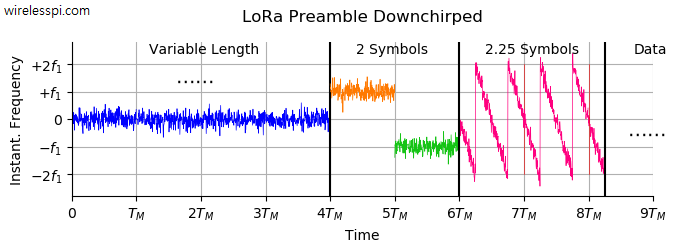
The noisy constant frequency part at the start (shown in blue) can be detected by monitoring the FFT output for a period of time until the same bin has the strongest magnitude for several consecutive symbols. This can only happen in a valid signal because
- white noise has a power spectral density that is constant over the whole spectrum and this randomness does not allow the same bin win each time, and
- after the start of the payload, the data symbols with different frequencies jump from one value to another, particularly because LoRa PHY supports a data whitening block that breaks series of identical bits and introduces randomness in the stream.
- Once the preamble is identified, the next question is to locate the exact sample as a starting index to the FFT input for detection of symbols. This is done by a Start of Frame Delimiter (SFD). As shown in the figure below, a simple solution to mark the SFD boundary is to multiply the preamble with an upchirp that cancels the downchirps at the end of the preamble and generates an (ideally) constant frequency.
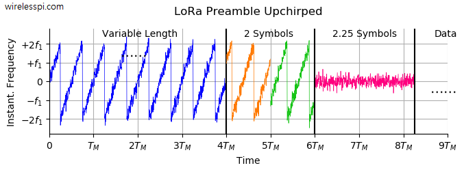
The FFT of this de-chirped portion of the signal can be taken for a window of $M$ samples as usual, say from sample number $n$ to $n+M-1$. However, instead of shifting through the whole block of next $M$ samples from $n+M$ to $n+2M-1$, the FFT input is the window of samples from $n+1$ to $n+M$. This is computationally expensive since each sample participates in multiple FFT operations. Nevertheless, once the exact start of the first data symbol is identified through the SFD boundary, the receiver can switch back to the regular operation of block-by-block FFTs corresponding to LoRa symbols. A clock recovery loop can then prevent this window from slipping away from the gradual build up of synchronization errors due to clock drift. The downchirps also prove useful for frequency synchronization through many OFDM-like algorithms.


Keep in mind that these synchronization techniques are simple from an algorithmic perspective but costly from a computational viewpoint. Elegant algorithms that are efficient to implement can be designed for a professional low-power radio by exploiting the vast resource of DSP knowledge applied to wireless communication receivers.
Concluding Remarks
This article presents a brief overview of Frequency Shift – Chirp Spread Spectrum (FS-CSS) modulation used in LoRa PHY. An instantaneous phase analogy with PSK can help the reader easily move to an instantaneous frequency signal of FS-CSS. Only simple signal detection and synchronization techniques are explained for experimental demodulation. To focus on the signal level details, further topics related to the data bits such as gray coding, data whitening, interleaving, forward error correction and packet headers are not investigated.


Very clear explanation and outstanding graphs.
Congrats
Glad that you liked the article.
Hi Qasim,
really great job rich in details and the necessary math. Very much appreciated ! The topic is not an easy one to get the grasp of !
I have one comment on equation (8):
TM=1/f1 . . .
how can that possibly be ? The signal with frequency f1 will cover several cycles/phases during TM and not just one ! Am I missing something ?
Many thanks for your valuable contribution
Best regards
Stefano
Great question. Please see Eq (6), where you will find that $f_1$ is not about cycles (remember they’re increasing or decreasing according to the chirp rate) but instead about the starting frequency that determines the modulation symbol.
Hi Qasim,
many thanks for your prompt reply. I got it now ! keep up with the good work and have a nice day.
best regards
stefano
I wish i was born a native English speaker. I am 54y old and i am very interested in understanding the IQ modulation (and others like LORA) but i have still difficulties to understand how IQ demodulation works. Ok, i make a signal with IQ modulator. But i feel that the demodulator local oscillator must be freq-synchronized from time to time and must be phase synchronized from time to time. Without this continuous synchronization, i cant imagine how the IQ receiver make that inphase signal and the other one. Sorry for my English, but it is more difficult to understand something if you were born with a very different language, so foreigners would need a more detailed explanation than native speakers. I like to understand the basic of IQ signal receiving first of all. Please help somehow !!! thank you !!!
I understand you want to build the concept right from the fundamentals.
i will try this two Links you sent, thanks, best wishes to you !!!
Hello,
I find the equation $T_M=\frac{M}{B}$ very confusing. It means that if the bandwidth increases, then my symbol time will be shorter. I understand that bandwidth is linked to data rate but on the other hand, by increasing bandwidth the ‘distance’ needed to go from low to high frequency is increased so it should take longer time. Where is my error in this interpretation ? Thanks a lot !
The error lies in the fact that one parameter has to be fixed. For your case, let’s consider the following.
Beautifully explained Qasim and I love the picture of the sunrise and analogy!
Thank you Dan 🙂
Dear Qasim,
Thank you very much for your insightful explanation. It was truly captivating and has piqued my curiosity about the detailed LoRa specifications. Could you please provide the specification document or a link related to the LoRa PHY layer? I would like to delve further into understanding LoRa.
Thank you!
Thank you. Since LoRa is a propriety modulation scheme, there is no open document available for this purpose. However, many people have reverse engineered the LoRa physical layer which you can find by searching for the expression ‘LoRa PHY’ in any search engine.
Dear Qasim,
Great work! I am just reading over some of the topics.
One question: How can you have $μ=B/T_M< 0$?
It is possible because the bandwidth $B$ in this linearly changing frequency signal is just the difference between the end frequency and the start frequency. In a decreasing frequency case, the end frequency is lesser than the start frequency and hence $\mu$ becomes negative.
Hey there,
I have demodulated the LoRa signal from the SX1276. After the initial 8 zero symbols, I am observing symbols 8 and 16 before the downchirps. The datasheet specifies the sync word as 0x12. Given that the spreading factor is 6, can someone help me validate the sync word from the LoRa symbols?
Is there any particular reason why all symbols on your diagrams are “rolled” by 180°?
I mean – on all waterfalls I’ve seen, (including my own captures of SX1262), preamble starts like ╱╱╱, not like ⸍╱╱⸝ and the transition between preamble and SOF looks like ╱╱╲╲, not like ⸍╱⸝⸜╲⸌.
Great comment. Thanks. What you’re looking at are real spectra from a certain frequency $F_0$ to $F_0+B$. What I draw here are complex spectra centered at 0 and the range is from $F_0-B/2$ to $F_0+B/2$. Both are fine but most DSP engineers like this baseband approach.