Frequency Modulation (FM) is as old as the history of wireless communications itself. The past few decades saw the rise of digital signal processing in all spheres of life that pervaded even the implementation of analog modulation schemes. Today many of the FM systems are built using discrete-time techniques instead of the conventional circuitry as described below.
Frequency Modulation
In digital communications, data is sent through altering a characteristic of an electromagnetic wave such as amplitude, frequency or phase in discrete steps (e.g., $M$ number of levels). Such systems are known as Amplitude Shift Keying (ASK), Frequency Shift Keying (FSK) and Phase Shift Keying (PSK), respectively. Analog modulation schemes, on the other hand, vary the desired parameter in a continuous fashion according to the message signal.
Frequency Modulated (FM) systems trade off bandwidth with power, i.e., they exhibit good noise performance at a cost of high bandwidth. This is why they are used in FM audio broadcasting and specialized point-to-point communication systems. We now turn towards how an FM modulator is implemented through DSP techniques.
Message Signal
The starting point is the familiar relation between the frequency $f$ and instantaneous phase $\theta(t) = 2\pi f t$ in a sinusoid. The frequency is defined as the rate of change of phase.
\[
f = \frac{1}{2\pi}\frac{d \theta(t)}{dt}
\]
This frequency needs not be constant at all times and can be represented as $f(t)$. As the frequency changes, the relation still holds true. In our scenario, the message signal, denoted by $x(t)$, can modulate the frequency variations in a carrier sinusoid. Therefore,
\[
x(t) = \frac{1}{2\pi}\frac{d \theta(t)}{dt}
\]
To find the phase $\theta(t)$ from here, we need to integrate both sides of the above equation starting with zero initial conditions at time $0$.
\begin{equation}\label{equation-fm-phase}
\theta(t) = 2\pi \int_{0}^t x(\tau) d\tau
\end{equation}
If the carrier wave is represented as
\[
y(t) = A_c \sin (2\pi f_c t),
\]
then the waveform for an FM signal is given by introducing the time-varying phase into the above expression.
$$\begin{equation}
\begin{aligned}
y(t) &= A_c \sin \big[2\pi f_c t + \theta(t)\big]\nonumber \\
&= A_c \sin \left[2\pi f_c t + 2\pi k_f \int_{0}^t x(\tau) d\tau\right]
\end{aligned}
\end{equation}\label{equation-fm-modulation}$$
where the phase $\theta$ has been replaced from Eq (\ref{equation-fm-phase}) that is multiplied with a new factor $k_f$, the frequency deviation constant.
Frequency Deviation
To understand what the frequency deviation means, consider the instantaneous phase expression in Eq (\ref{equation-fm-modulation}).
\begin{equation}\label{equation-fm-carrier-phase}
\theta_c(t) = 2\pi f_c t + 2\pi k_f \int_{0}^t x(\tau) d\tau
\end{equation}
The instantaneous frequency is thus given by
\[
f(t) = \frac{1}{2\pi}\frac{d \theta_c(t)}{dt} = f_c + k_f x(t)
\]
This equation shows that the instantaneous frequency varies according to the message signal scaled by the frequency deviation. The maximum deviation of this frequency occurs for the maximum value of $|x(t)|$. Denoting this value by $A_m$, we get the peak frequency deviation.
\begin{equation}\label{equation-frequency-deviation}
\Delta f = k_f A_m
\end{equation}
Peak frequency deviation represents how far the modulated signal frequency can stretch in either direction as compared to the carrier frequency. Note that it depends on the frequency deviation constant as well as the peak amplitude of the input signal.
Next, we turn our attention towards the modulation index.
Modulation Index
Consider a sinusoidal message signal written as
\[
x(t) = A_m \cos \left(2\pi f_m t \right)
\]
Plugging this expression into Eq (\ref{equation-fm-modulation}), we get
\[
\begin{aligned}
y(t) &= A_c \sin \left[2\pi f_c t + 2\pi k_f \frac{A_m}{2\pi f_m} \sin \left(2\pi f_m t \right)\right] \\\\
&= A_c \sin \Big[2\pi f_c t + \beta \sin \left(2\pi f_m t \right)\Big]
\end{aligned}
\]
In the above expression, the parameter $\beta$ is the FM modulation index defined as
\[
\beta = \frac{k_f A_m}{f_m}
\]
If it is scaled by the maximum value in the message signal $A_m$, the modulation index can be interpreted as the normalized frequency deviation, where this normalization is with respect to the maximum frequency in the message signal. This is where the ideas of narrowband FM and wideband FM arise where a small modulation index $\beta << 1$ indicates narrowband FM while a large $\beta$ represents wideband FM.
For a non-sinusoidal signal, the FM modulation index is written as
\[
\beta = \frac{k_f A_m}{B} = \frac{\Delta f}{B}
\]
where $B$ is the bandwidth of the message signal $x(t)$, $A_m$ is its maximum value in absolute sense and $\Delta f$ is $k_f A_m$ as in Eq (\ref{equation-frequency-deviation}). But how much is the bandwidth $B$ occupied by an FM signal?
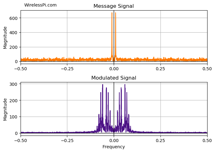
FM Bandwidth
FM signals are non-linear and hence there is no straightforward way to derive the occupied bandwidth. As an approximation, Carson’s rule gives the effective bandwidth of an FM signal that is determined on the basis of $98\%$ bandwidth occupancy.
\[
B_{\text{FM}} = 2(\beta+1)B = 2(\Delta f+B)
\]
where $B$ is the message signal bandwidth and $\beta$ is defined in the last equation above. The spectra of the message signal and the modulated signal are plotted in the figure below.
For example, in commercial FM broadcasts, the audio signal has a maximum frequency of approximately $f_m=15$ kHz while the peak frequency deviation is $75$ kHz. From Carson’s rule, the bandwidth can be approximated as
\[
B_{\text{FM}} = 2\left(\frac{75}{15}+1\right)15 = 180 ~\text{kHz}
\]
If an AM system was used to transmit the same information, the bandwidth required would only be twice the audio signal bandwidth, or $30$ kHz. While worse than Amplitude Modulated (AM) systems in terms of bandwidth and Rx complexity, FM signals enjoy certain advantages for which this is a worthwhile price to pay.
- Noise in communication systems impact the amplitude of a wireless signal differently as compared to its frequency. Since an AM signal carries information in its amplitude, any amplitude perturbations affect the AM demodulator performance and make it vulnerable to amplitude noise and interference.
On the other hand, an FM signal carries information in instantaneous frequency, so amplitude noise is less directly mapped into the frequency of baseband signal. Also, FM receivers often include limiters that remove amplitude variations before FM demodulation, making FM robust to many amplitude disturbances. This results in better signal fidelity suited to high-quality broadcasting systems.
- Since the variations in the message are encoded into signal frequency but not the amplitude, the modulation signal has a constant envelope that can be transmitted with efficient non-linear amplifiers.
With continuous-time details covered, we can easily translate this process into a digital FM modulator.
Discrete-Time Implementation
The modulation phase in Eq (\ref{equation-fm-phase}) is a continuous-time description of the modulation process. For a discrete-time implementation, we need to sample this signal after including the frequency deviation $k_f$.
$$\begin{equation}
\begin{aligned}
\theta(nT_s) &= 2\pi k_f \int_{0}^{nT_s} x(\tau) d\tau \\
&= 2\pi k_f \int_{0}^{(n-1)T_s} x(\tau) d\tau + 2\pi k_f \int_{(n-1)T_s}^{nT_s} x(\tau) d\tau \\ \\
&=\theta[(n-1)T_s] + 2\pi k_f T_s x[(n-1)T_s]
\end{aligned}
\end{equation}\label{equation-fm-phase-baseband}$$
where the continuous-time integral has been replaced with the backward difference version of a discrete-time integrator. A block diagram of a discrete-time FM modulator is now drawn in the figure below where $D$ denotes a unit time delay commonly written as $z^{-1}$. The diagram includes the complete instantaneous phase in the carrier signal, see Eq (\ref{equation-fm-carrier-phase}). The Look-Up Table (LUT) stores the values of cosine and sine functions. The complete setup forms a Numerically Controlled Oscillator (NCO) for FM signal generation. The NCO combined with a Digital to Analog Converter (DAC) turns into a Direct Digital Synthesizer (DDS) implementation.
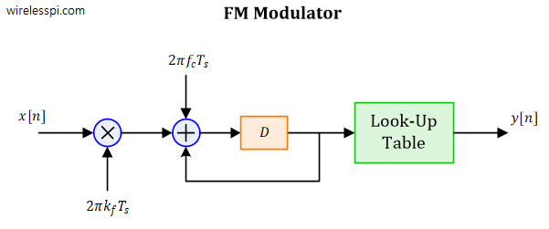
Analogous to Eq (\ref{equation-fm-modulation}), the output $y[n]$ is a complex exponential at a frequency $f_c$ that is written as
\begin{equation}\label{equation-discrete-fm}
y[n] = A_c e^{j\left[2\pi f_c nT_s + \theta(nT_s)\right]}
\end{equation}
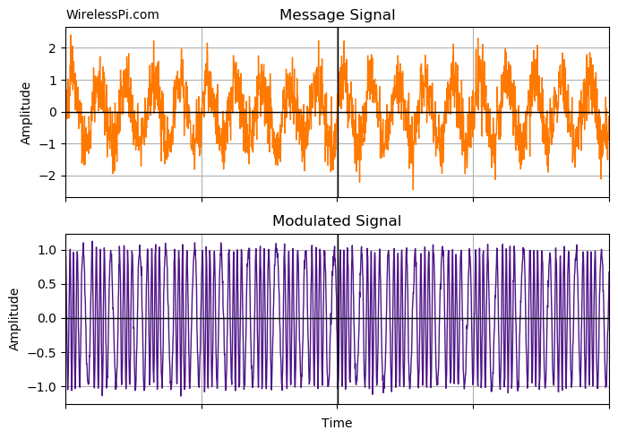
An example FM signal with a noisy message signal of frequency 1 KHz, frequency deviation 2.5 kHz and a carrier frequency of 5 kHz is plotted in the figure below (only the real part is shown). Observe the frequency variations in the modulated signal according to the message signal.
We now see how this signal can be demodulated using digital signal processing techniques.
FM Demodulation
To focus on the signal processing operations, let us remove the carrier term by multiplying $y[n]$ in Eq (\ref{equation-discrete-fm}) with $e^{-j2\pi f_c nT_s}$ and assume that $A_c$ is equal to 1 for simplicity.
\[
z[n] = y[n]e^{-j2\pi f_c nT_s} = e^{j\theta(nT_s)}
\]
What remains is a complex exponential with the discrete-time phase from Eq (\ref{equation-fm-phase-baseband}).
\begin{equation}\label{equation-fm-demodulation}
z[n] = e^{j\theta(nT_s)} = e^{j \left\{\theta[(n-1)T_s] + 2\pi k_f T_s x[(n-1)T_s]\right\}}
\end{equation}
From here, the FM demodulation techniques can be divided into three different categories.
- Differentiate and access phase
- Access phase and differentiate
- Phase-Locked Loop (PLL)
We describe each of these categories in detail next.
1. Differentiate and Access Phase
A conventional demodulation technique used in old analog FM receivers is to differentiate the FM signal $y(t)$ in Eq (\ref{equation-fm-modulation}).
\[
\dot y(t) = A_c \left[2\pi f_c + 2\pi k_f \cdot x(t)\right]\cos \left[2\pi f_c t + 2\pi k_f \int_{0}^t x(\tau) d\tau\right]
\]
After passing through a DC blocker, this process renders the message signal $x(t)$ as envelope variations of the derivative (sinusoidal) signal. An envelope detector can then track these changes to reproduce $x(t)$ at the receiver.
In discrete domain, this would be an inefficient method to demodulate an FM signal. But something that closely resembles this technique can be implemented. For this purpose, consider the block diagram below where $D$ denotes a unit time delay, commonly shown as $z^{-1}$.
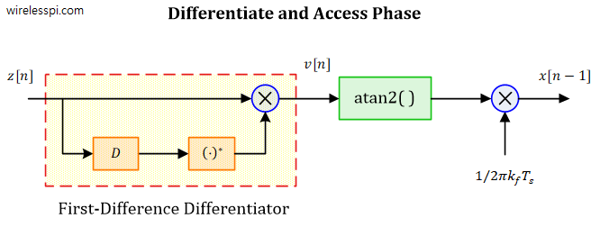
What happens when the above signal is multiplied with a delayed and conjugated version of itself? Since a conjugate operation reverses the phase sign, we have
\[
v[n] = e^{j\theta(nT_s)}\cdot e^{-j\theta[(n-1)T_s]} = e^{j\left\{\theta(nT_s) – \theta[(n-1)T_s]\right\}}
\]
We deduce that conjugate multiplication computes the difference between phases. Apparently, this is a delayed conjugate product operation used in many signal processing applications. Behind the scene, this is an implementation of a discrete-time first-difference differentiator.
Using Eq (\ref{equation-fm-demodulation}) in the above expression and taking the angle through atan2( ) operation or an approximation of atan2( ), we can write
\[
\measuredangle v[n] = 2\pi k_f T_s \cdot \underbrace{x[(n-1)T_s]}_{\text{Message Signal}}
\]
which is our desired message signal delayed by one time unit and scaled by $2\pi k_f T_s$.
\[
x[(n-1)T_s] = \frac{1}{2\pi k_f T_s}\measuredangle v[n]
\]
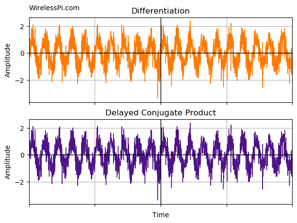
The demodulated waveform for an FM signal is shown in the figure below.
The above $\measuredangle$ operation is the familiar $\arg()$ function in mathematics, implemented by atan2() in programming languages. Computing this value is resource intensive. But there is a way to avoid this computation if the sample rate is high enough.
Consider the differentiated (delay-and-conjugate multiplication) signal $v[n]$ above, the argument of which is given by
\[
\Delta_\theta = \theta[n] – \theta[n-1]
\]
Now at a high sample rate, this phase will not change much from one sample to the next. We then have
\[
\begin{aligned}
e^{j\Delta_\theta} &= \cos \Delta_\theta + j\sin \Delta_\theta \\
&\approx 1 + j\Delta_\theta \qquad \rightarrow \qquad \text{for small } \Delta_\theta
\end{aligned}
\]
In words, for a high sample rate, just taking the imaginary component of $v[n]$ bypasses computing the argument. How high this sample rate needs to be depends on the tolerance allowed by the system design. As a rough estimate, sampling at a rate between 6 to 10 times the Nyquist rate seems to do the trick.
While this is a simple procedure, the first-difference differentiator suffers from a performance penalty due to excessive noise. We describe an improved technique for FM demodulation next.
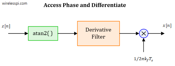
2. Access Phase and Differentiate
The above technique computes the derivative (first difference) first and accesses the phase next. A better technique is to access the phase first and then compute the derivative with a superior filter. There are two routes to this end.
- Consider the signal $z[n]$ in Eq (\ref{equation-fm-demodulation}) and access its phase through an atan2( ) operation.
\[
\measuredangle z[n] = \theta(nT_s)
\]As shown earlier in Eq (\ref{equation-fm-phase}), the derivative of this phase is our desired message signal $x[n]$. In practice, this derivative is computed through a derivative FIR filter with impulse response $h[n]$ that can be computed through a variety of techniques (see the design of a discrete-time differentiator for details). This is convolved with the signal phase as
\[
x[n] = \frac{1}{2\pi k_f T_s} \Big\{\theta(nT_s)*h[n] \Big\}
\]A block diagram of this procedure is drawn in the figure below.

Again, it is of utmost importance to unwrap the phase after extraction to get a valid result. This technique is more suited to FPGA implementations where a CoRDiC routine can be pipelined for a faster output.
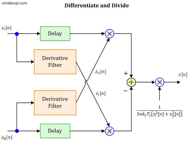
- From a DSP (Digital Signal Processor) implementation perspective, the phase access and derivative operation can be simplified as follows.
Start with expressing the signal $z[n]=e^{j\theta(nT_s)}$ in its real (in-phase) and imaginary (quadrature) components.
\[
z(nT_s) = z_I(nT_s) + jz_Q(nT_s)
\]The phase $\theta(nT_s)$ is then given by
\[
\theta(nT_s) = \tan^{-1}\left[\frac{z_Q(nT_s)}{z_I(nT_s)}\right]
\]Consider the following trigonometric identity.
\[
\frac{d}{dx}\left[ \tan^{-1}(x)\right] = \frac{1}{1 + x^2}
\]Using this identity, the derivative of $\theta(nT_S)$ can be written as
\[
\dot \theta(nT_s) = \frac{d}{dt} \tan^{-1}\left[\frac{z_Q(nT_s)}{z_I(nT_s)}\right] = \frac{1}{1+z_Q^2(nT_s)/z_I^2(nT_s)} \frac{d}{dt}\left[\frac{z_Q(nT_s)}{z_I(nT_s)}\right]
\]Next, we can simplify the above expression as
\[
\dot \theta(nT_s) = \frac{z_I^2(nT_s)}{z_I^2(nT_s)+z_Q^2(nT_s)}\frac{z_I(nT_s)\dot z_Q(nT_s) – z_Q(nT_s)\dot z_I(nT_s)}{z_I^2(nT_s)}
\]This generates our final relation as
\[
\dot \theta(nT_s) = \frac{z_I(nT_s)\dot z_Q(nT_s) – z_Q(nT_s)\dot z_I(nT_s)}{z_I^2(nT_s)+z_Q^2(nT_s)}
\]A block diagram of this approach is shown in the figure below.
Note the following in this figure.
- There is no atan2( ) computation that gives rise to extra complexity in the algorithm.
- As with the previous atan2 + differentiate approach, the derivative here can be implemented with an FIR filter.
- In this technique, it is imperative to design an FIR differentiator with an odd number of taps. The reason is to align the signals in the two parallel branches with each other as the group delay of an FIR filter of length $N$ is given by
\[
\text{Group Delay} = \frac{N-1}{2}
\]With an odd number of taps the delay in the FIR differentiator is an integer number of samples. Therefore, the Delay block above is simply an integer number of samples. In a practical implementation, the first and last $(N-1)/2$ samples from the differentiator are removed to automatically obtain alignment with $z_I[n$] and $z_Q[n]$.


We now move towards our third and final approach for DSP-based FM demodulation.
3. Phase-Locked Loop (PLL)
A discrete-time Phase-Locked Loop (PLL) that is used for carrier and clock synchronization in Software Defined Radios (SDR) can also be employed to demodulate an FM signal. A block diagram of such an approach is shown in the figure below where the input signal $s[n]$ can be replaced with our input signal $z[n]$ in this case. Just like a carrier PLL tracks the phase and frequency of an incoming sinusoid, the same PLL can track the frequency of an FM modulated signal and automatically performs the demodulation in this process.
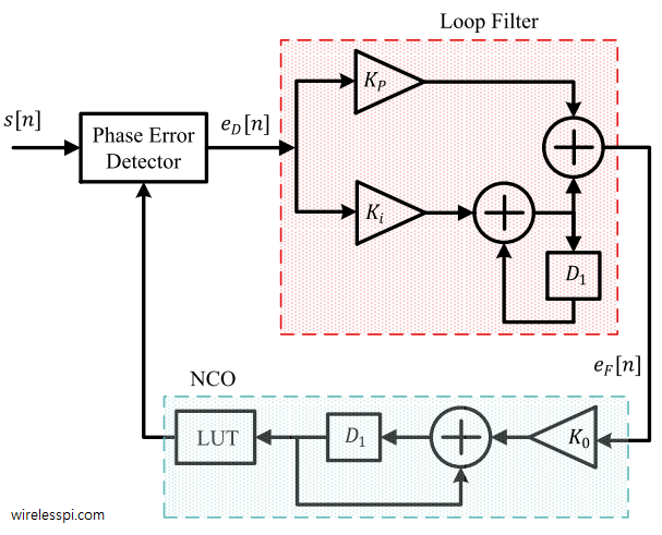
The loop constants in the above Proportional-plus-Integrator (PI) filter can be computed as described in the PLL in an SDR context. The main problem with this approach is the need for a large lookup table for Direct Digital Synthesis (DDS) to store samples of sines and cosines.
Conclusion
Three different approaches for FM demodulation in DSP based systems are described, namely differentiate and then access the phase, access the phase and then differentiate and a PLL. The atan2( ) and differentiator approach, along with its derivative FIR filters, give the best results in terms of complexity and output SNR performance. To implement the digital version of FM, see FSK (Frequency Shift Keying) in the open-source GNU Radio framework and how to demodulate a CQPSK signal using a C4FM receiver


Super and thank you.
Thank you very much for things that your knowledge brought to me.
I wonder if I want to dive into FSK related technique. Which of your documents or books… I can refer to?
Thank you very much
I appreciate your kind words. I have mostly focused on linear modulation techniques. But there are two ways in which my book Wireless Communications from the Ground Up can help you.
Hope that helps.
I am trying to mux 2 different types of modulations: 8VSB and OFDM, each with 6 MHz BW. The candidates are LDM and TDM with LDM probably the issue will be the SNR and TDM, the issue will be the loss of frames. Any idea on the feasibility? If yes, the 8VSB is using TS while OFDM can use either TS or IP packets
It depends on lots of factors. I haven’t covered LDM in detail yet but I would be cautious to overlap any other format with OFDM for LDM, since its PAPR is already quite high. I don’t see why a well-designed TDM system would suffer from a loss of frames.
For Eductionaal purpose
Very nice super helpful.
An excellent dive into frequency modulation and demodulation using DSP techniques! The blog is detailed and informative, making complex concepts easy to grasp. Great work by the author in making this topic so accessible!