When we think about signal processing, the focus is usually magnitude response of a system. However, in several DSP applications, the signal phase holds as much, if not more, significance as the magnitude response. For example, in digital FM demodulation, carrier phase synchronization and RF ranging, the phase (found through arctangent in four quadrants) of a complex signal needs to be computed by an FPGA or a DSP for further processing. In image processing applications, such an operation is also required to calculate the gradient orientations used in several popular feature descriptors like the Scale-Independent Feature Transform (SIFT) or the histograms of oriented gradient.
Let us define a four-quadrant inverse tangent before turning towards how this can be accomplished through a few different techniques.
Four-Quadrant Inverse Tangent
Consider a complex number $z$ with a real component $x$ and imaginary component $y$.
\[
z = x+j\; y
\]
Denote the magnitude of $z$ as $|z|=r$ and the angle $\measuredangle z=\theta$. A four-quadrant inverse tangent operation, implemented in numerical computing platforms as $\theta$ $=$ atan2$ (y,x)$, is not the same as $\tan^{-1} y/x$. This is because
\begin{align*}
\tan^{-1} \frac{+y}{+x} ~&=~ \tan^{-1} \frac{-y}{-x} \quad \rightarrow \quad \text{in}~ [0,+\pi/2],~ \text{Quadrant I} \\
\tan^{-1} \frac{-y}{+x} ~&=~ \tan^{-1} \frac{+y}{-x} \quad \rightarrow \quad \text{in}~ [0,-\pi/2],~ \text{Quadrant IV}
\end{align*}
In words, there is no way to differentiate whether the complex number $z$ lies in quadrant I or III. The same holds for $z$ lying in quadrant II or IV. On the other hand, the angle $\theta$ should be in the range $[-\pi,\pi)$ because
- Quadrant I: $\theta$ should be in $[0,\pi/2]$
- Quadrant II: $\theta$ should be in $[\pi/2,\pi]$
- Quadrant III: $\theta$ should be in $[-\pi/2,-\pi]$
- Quadrant IV: $\theta$ should be in $[0,-\pi/2]$
In addition, the following four cases need to be considered as well.
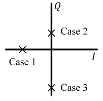
- Case 1: When $x<0$ and $y=0$, $\theta$ should be $\pi$, not $0$
- Case 2: When $x=0$ and $y>0$, $\theta$ should be $+\pi/2$
- Case 3: When $x=0$ and $y<0$, $\theta$ should be $-\pi/2$
- Case 4: When $x=0$ and $y=0$, $\theta$ should be undefined.
Taking into account all four quadrants, $\measuredangle z=\theta$ is defined in terms of $\tan^{-1} (y/x)$ as
\theta = \text{atan2}(y,x) =
\begin{cases}
\tan^{-1} \frac{y}{x} & x > 0 \\
\tan^{-1} \frac{y}{x} + \pi & x < 0 \mbox{ and } y \ge 0\\ \tan^{-1} \frac{y}{x} - \pi & x < 0 \mbox{ and } y < 0\\ +\pi/2 & x = 0 \mbox{ and } y > 0\\
-\pi/2 & x = 0 \mbox{ and } y < 0 \\ \mbox{undefined } & x = 0 \mbox{ and } y = 0. \end{cases} \end{equation}
A straightforward way to implement such a function in any digital processor is to write a simple program satisfying the above conditions, in which the function $\tan^{-1}(~)$ is approximated through its power series. Let $v = y/x$, then we have
\[
\tan^{-1}(v) = v \;- \frac{v^3}{3} + \frac{v^5}{5} – \frac{v^7}{7} + \cdots
\]
where the series can be truncated to a desired accuracy. However, this approach is slow to converge, exhibits error growth and requires several terms to achieve sufficient accuracy.
Next, we describe some techniques that compute the four-quadrant inverse tangent in an efficient manner.
Hardware Implementation
For hardware computation, the most widely used techniques are as follows.
Lookup Table (LUT)
In applications where sufficient memory is available and the number of computations needs to be minimized, precomputed values of the four-quadrant inverse tangent atan2( ) can be stored in a large lookup table in the processor memory. During the execution of any algorithm, the right value can be easily retrieved on runtime from a memory address.
It is usually impossible to store a lookup table that satisfies the desired resolution in fixed point. For this purpose, interpolation between existing values can be used to get more accurate results. This is a tradeoff between saving memory at the expense of a few computations for interpolation per output sample.
Coordinate Rotation Digital Computer (CoRDiC)
Coordinate Rotation Digital Computer (CoRDiC) is a simple and efficient algorithm that is widely used in real-time digital signal processing applications. It computes several functions through only additions and shift operations, such as trigonometric and hyperbolic functions, multiplications, divisions, exponentials, logarithms and square roots. The four-quadrant inverse tangent atan2( ) can also be calculated using the same approach, particularly in systems where CoRDiC is alrealy used for implementing one or more of other functions mentioned above.
Polynomial Approximations
One technique can be to approximate an arctangent function first, which can then be plugged in $\text{Eq}~(\ref{equation-atan2})$ to calculate the four-quadrant inverse tangent. As an example [1],
\[
\tan^{-1}\frac{y}{x} = \frac{xy}{x^2 + 0.28125y^2}
\]
The range of this approximation is $-\pi/4 \le \theta \le +\pi/4$ radians while the maximum error is $0.0045$ radians. This expression can be extended to cover the full range $-\pi$ to $\pi$ through incorporating rotational symmetry properties of the arctangent. The algorithm is particularly suitable for applications where $x^2$ and $y^2$ are already computed during the implementation of demodulation or Automatic Gain Control (AGC) algorithms.
The main drawback of this approach is that multiple checks and adjustments are required to make it work as an atan2( ) function that is not suited to computations within a single instruction cycle.
Better approximations also exist [2] such as
\[
\tan^{-1}\frac{y}{x} = \frac{c\cdot xy+y^2}{x^2+2c\cdot xy + y^2}
\]
where $c$ is a constant given by $0.596227$. The range of this approximation is $0 \le \theta \le +\pi/2$ radians while the maximum error is $0.0028$ radians. This technique is also more easily generalized to four quadrants.
In a fixed-point implementation, the range of division $y/x$ can be outside the allotted range and some kind of normalization is necessary. Another example of such normalization is FM demodulation in which amplitude variations should be removed before accessing the phase for frequency detection. In these situations, another technique presented in [3] works as follows.
- For Quadrant I, compute the ratio
\[
\gamma = \frac{x-y}{x+y}
\]The angle can then be computed through linear approximation as
\[
\theta = a_0-a_0\gamma
\]where $a_0=\pi/4$. Negate this value if the complex number $z$ lies in Quadrant IV.
- For Quadrant II, compute the ratio
\[
\gamma = \frac{x+y}{y-x}
\]The angle can then be computed through linear approximation as
\[
\theta = 3a_0-a_0\gamma
\]Negate this value if the complex number $z$ lies in Quadrant III.
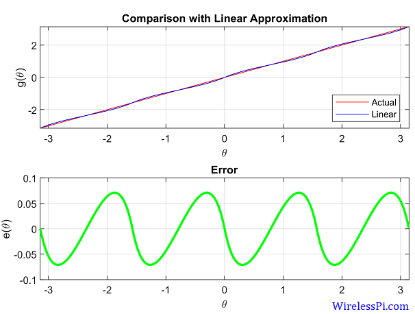
A plot of the error between the actual atan2( ) and the linear approximation is shown below. Observe the maximum error of $0.07$ radians at a few locations.

If better accuracy is desired, a higher-order approximation such as a cubic one can be employed as follows.
- For Quadrant I,
\[
\theta = a_3\gamma^3 -a_1\gamma + a_0
\]where $a_3=\pi/16$, $a_1=5\pi/16$ and $a_0=\pi/4$. Negate this value if the complex number $z$ lies in Quadrant IV.
- For Quadrant II,
\[
\theta = a_3\gamma^3 -a_1\gamma + 3a_0
\]Negate this value if the complex number $z$ lies in Quadrant III.
A plot of the error between the actual atan2( ) and the cubic approximation is shown below. Observe the maximum error of $0.01$ radians at a few locations.

Conclusion
In conclusion, the lookup table method is the best for atan2( ) computation in terms of speed, the polynomial approximation in terms of simplicity while the CoRDiC for efficiency and versatility.
References
[1] R. Lyons, Another Contender in the Arctangent Race, IEEE Signal Processing Magazine, 2004.
[2] X. Girones, C. Julia, D. Puig, Full Quadrant Approximations for the Arctangent Function, IEEE Signal Processing Magazine, 2013.
[3] FM Demodulation Using a Digital Radio and Digital Signal Processing, James Michael Shima, University of Florida, 1995.