In the discussion on piecewise polynomial interpolation, we emphasized on the fact that the fractional interval $\mu_m$ needs to be updated for each symbol time $mT_M$ and hence the subscript $m$ in $\mu_m$. For this reason, the interpolation process becomes a two-step procedure.
- Update the filter coefficients $h_p[n]$.
- Perform the convolution between $z(nT_S)$ and $h_p[n]$.
This process can be simplified if the two steps above can be combined in such a way that $\mu_m$ update is weaved into the convolution operation. In other words, instead of a two-input hardware multiplication with two variable quantities, complexity can be reduced by restructuring the problem such that one input in the two-input hardware multiplication remains fixed. This is accomplished by separating the constant factors from the powers of $\mu_m$ in filter equations, which is discussed in detail below.
Cubic Interpolation
Odd degree polynomials approximate the interpolant by using an even number of samples that ensures the linear phase property. After $p=1$, the next odd degree polynomial is with $p=3$ and is known as cubic interpolation. Plugging $p=3$ in the interpolation equation,
\[
z(t) \approx c_p t^p + c_{p-1}t^{p-1} + \cdots + c_1 t + c_0
\]
we get
\begin{equation*}
z(t) \approx c_3t^3 + c_2 t^2 + c_1 t + c_0
\end{equation*}
Therefore,
\begin{align}
z(nT_S+\mu_m T_S) &\approx c_3 (nT_S+\mu_m T_S)^3 + c_2 (nT_S+\mu_m T_S)^2 + \nonumber \\
&\hspace{1.7in}c_1 (nT_S+\mu_m T_S) + c_0 \label{eqTimingSyncCubicInterpolation1}
\end{align}
Following the same derivation as in linear interpolation, the coefficients $c_3$, $c_2$, $c_1$ and $c_0$ need to be found every time $\mu_m$ changes. The four samples around the interpolant are given by
\begin{align*}
z((n-1)T_S) &= c_3((n-1)T_S)^3 + c_2((n-1)T_S)^2 + c_1(n-1)T_S + c_0 \\
z(nT_S) &= c_3(nT_S)^3 + c_2 (nT_S)^2 + c_1 nT_S+c_0 \\
z((n+1)T_S) &= c_3((n+1)T_S)^3 + c_2((n+1)T_S)^2 + c_1(n+1)T_S + c_0 \\
z((n+2)T_S) &= c_3((n+2)T_S)^3 + c_2((n+2)T_S)^2 + c_1(n+2)T_S + c_0
\end{align*}
These are four equations with four unknowns that can be easily solved to compute $c_3$, $c_2$, $c_1$ and $c_0$. Substituting them back in Eq~\eqref{eqTimingSyncCubicInterpolation1} yields
\begin{aligned}
z(nT_S+\mu_m T_S) &= \left(\frac{\mu_m^3}{6}- \frac{\mu_m}{6} \right)z((n+2)T_S) + \\
&\hspace{0.2in} \left(-\frac{\mu_m^3}{2}+\frac{\mu_m^2}{2}+\mu_m \right)z((n+1)T_S) + \\
&\hspace{0.2in} \left(\frac{\mu_m^3}{2}-\mu_m^2-\frac{\mu_m}{2}+1 \right) z(nT_S) + \\
&\hspace{0.2in} \left(-\frac{\mu_m^3}{6}+\frac{\mu_m^2}{2} – \frac{\mu_m}{3} \right) z((n-1)T_S)
\end{aligned}
\end{equation}\label{eqTimingSyncCubicInterpolation2}$$
As before, the desired interpolant can again be written as the output of a filter as
\begin{align}
z(nT_S+\mu_m T_S) &= h_3[-2] z((n+2)T_S) + h_3[-1] z((n+1)T_S) + \nonumber\\
&\hspace{1.3in}h_3[0] z(nT_S) + h_3[1] z((n-1)T_S) \nonumber\\
&= \sum \limits _{i=-2} ^1 h_3[i] z((n-i)T_S) \label{eqTimingSyncCubicFiltering}
\end{align}
where the filter coefficients are given by
$$ \begin{equation}
\begin{aligned}
h_3[-2] &= \frac{\mu_m^3}{6}- \frac{\mu_m}{6} \\
h_3[-1] &= -\frac{\mu_m^3}{2}+\frac{\mu_m^2}{2}+\mu_m\\
h_3[0] &= \frac{\mu_m^3}{2}-\mu_m^2-\frac{\mu_m}{2}+1\\
h_3[1] &= -\frac{\mu_m^3}{6}+\frac{\mu_m^2}{2} – \frac{\mu_m}{3}
\end{aligned}
\end{equation}\label{eqTimingSyncCubicFilter}$$
In the above equations, the subscript $3$ denotes cubic interpolation as $p=3$. An example of cubic interpolation is drawn in the figure below.

Observe how the curve has been smoothed out as compared to linear interpolation. This gain comes at a price of higher computational complexity paid for cubic interpolation.
Simplification through Farrow Technique
Begin with filter coefficients from cubic interpolation in Eq (\ref{eqTimingSyncCubicFilter}) and rewrite it as
\begin{align*}
h_3[-2] &= \frac{1}{6}\mu_m^3 + 0\cdot\mu_m^2 – \frac{1}{6}\mu_m + 0 \\
&= b_3[-2]\mu_m^3 + b_2[-2]\mu_m^2 +b_1[-2]\mu_m^1 + b_0[-2]\mu_m^0 = \sum \limits_{l=0}^{3} b_l[-2]\mu_m^l
\end{align*}
where $b_3[-2] = 1/6$, $b_2[-2]=0$, etc. Similarly, for other coefficients, we can write
\begin{align*}
h_3[-1] &= -\frac{1}{2}\mu_m^3+\frac{1}{2}\mu_m^2+1\cdot\mu_m + 0 = \sum \limits_{l=0}^{3} b_l[-1]\mu_m^l \\
h_3[0] &= \frac{1}{2}\mu_m^3-1\cdot\mu_m^2-\frac{1}{2}\mu_m+1 = \sum \limits_{l=0}^{3} b_l[0]\mu_m^l \\
h_3[1] &= -\frac{1}{6}\mu_m^3+\frac{1}{2}\mu_m^2 – \frac{1}{3}\mu_m+0 = \sum \limits_{l=0}^{3} b_l[1]\mu_m^l
\end{align*}
In general,
\begin{equation*}
h_3[i] = \sum \limits_{l=0}^{3} b_l[i]\mu_m^l
\end{equation*}
Observe that $b_l[i]$ are fixed coefficients independent of $\mu_m$ in the above expression and are given in the table below.

With this understanding in place, the filtering process from Eq (\ref{eqTimingSyncCubicFiltering}) can be rearranged such that convolution of the matched filter output is performed with the fixed coefficients $b_l[i]$.
\begin{align*}
z(nT_S+\mu_m T_S) &= \sum \limits _{i=-2} ^1 h_3[i] z((n-i)T_S)\\
&= \sum \limits _{i=-2} ^1 \cdot \sum \limits_{l=0}^{3} b_l[i]\mu_m^l \cdot z((n-i)T_S)\\
&= \sum \limits_{l=0}^{3}\mu_m^l \underbrace{\sum \limits _{i=-2} ^1 b_l[i] \cdot z((n-i)T_S)}_{y(l)}\\
&= \sum \limits_{l=0}^{3} y(l) \mu_m^l
\end{align*}
To obtain a hardware efficient filter structure known as Farrow structure, the above expression can be opened as
\begin{align*}
z(nT_S+\mu_m T_S) &= y(3)\mu_m^3 + y(2)\mu_m^2 + y(1)\mu_m^1 + y(0)\mu_m^0\\
&= \Big\{y(3)\mu_m^2 + y(2)\mu_m + y(1)\Big\}\mu_m + y(0)
\end{align*}
One more such step produces the Farrow structure for a cubic interpolator.
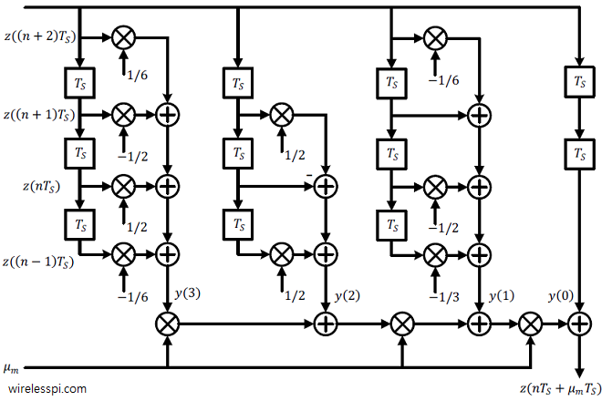
z(nT_S+\mu_m T_S) = \bigg\{\Big\{y(3)\mu_m +y(2)\Big\}\mu_m + y(1)\bigg\}\mu_m + y(0)
\end{equation}
The Farrow structure for cubic interpolation is drawn in the figure below where $T_S$ is a sample delay. Notice the fixed coefficients $b_l[i]$ operating on the matched filter output samples while a changing $\mu_m$ operates on the subsequent output $y(l)$. Although its block diagram looks complicated, the expression above is quite simple. Click on the figure to see the enlarged image.

A similar strategy can be applied to devise Farrow structures for polynomial interpolation for the cases when $p \neq 3$. For example, for $p=2$, it is given by
\begin{equation*}
z(nT_S+\mu_m T_S) = \Big\{y(2)\mu_m +y(1)\Big\}\mu_m + y(0)
\end{equation*}
This is a concise but very clear explanation, very helpful overview.