Discrete-Time Integrators

An integrator is a very important filter that proves useful in implementation of many blocks of a communication receiver such as symbol timing synchronization and Phase-Locked Loop (PLL). It is an inverse operation to a differentiator that is also used in many signal processing applications such as FM demodulation and image processing.

In continuous-time case, an integrator finds the area under the curve of a signal amplitude. A discrete-time system deals with just the signal samples and hence a discrete-time integrator serves the purpose of collecting a running sum of past samples for an input signal. Looking at an infinitesimally small scale, this is the same as computing the area under the curve of a signal sampled at an extremely high rate. For this discussion, a normalized sample time $T_s =1$ is assumed if it is not explicitly specified.

The starting point is the Laplace Transform $X(s)$ of a signal $x(t)$. The integral of such a signal is given by
\[
\begin{aligned}
x(t) \quad &\longleftrightarrow \quad X(s) \\
y(t) = \int x(t) dt \quad & \longleftrightarrow \quad Y(s) = \frac{1}{s}X(s)
\end{aligned}
\]

For an input $s[n]$ and output $r[n]$ with z-Transforms $S(z)$ and $R(z)$, respectively, there are three main methods to implement a discrete-time integrator.

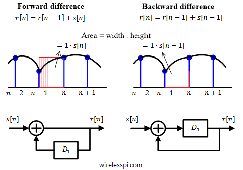
Forward difference

---

In a forward difference integrator, the term $1/s$ in Laplace domain is replaced by $T_s/(1-z^{-1})$ in z-domain.
\[
\begin{aligned}
R(z) = \frac{T_s}{1-z^{-1}}S(z) \\
R(z)(1-z^{-1}) = T_s\cdot S(z)
\end{aligned}
\]

Using the time-delay property of z-Transform, we get
\[
r[n] – r[n-1] = T_s\cdot s[n], \qquad \text{or} \qquad r[n] = r[n-1]+T_s\cdot s[n]
\]

Another way to see the forward difference integrator is through the following equation.
\begin{align}
r[n] &= T_s\sum _{i=-\infty}^{n} s[i] \nonumber \\
&= T_s\sum _{i=-\infty}^{n-1} s[i] + T_s\cdot s[n] \nonumber \\
&= r[n-1] + T_s\cdot s[n] \label{eqIntroductionForwardIntegrator}
\end{align}

For obvious reasons, the running sum $r[n-1]$ is a common component in all types of integrators; the differentiating factor is the term added to $r[n-1]$ as a replacement for area under the curve. For a forward difference integrator, this additional term is $s[n]$ — the current input. This is drawn in Figure below for $T_s=1$. Notice that the forward difference integrator computes its output after the arrival of the current sample, i.e., at time $n$.

The block diagram shown in the figure is used to implement a forward difference integrator in loop filter portion of a Phase Locked Loop (PLL) that is employed in carrier phase and symbol timing synchronization systems of a digital communication system.

Backward difference

---

In a backward difference integrator, the term $1/s$ in Laplace domain is replaced by $T_s z^{-1}/(1-z^{-1})$ in the z-domain.
\[
\begin{aligned}
R(z) = \frac{T_sz^{-1}}{1-z^{-1}}S(z) \\
R(z)(1-z^{-1}) = T_sz^{-1}S(z)
\end{aligned}
\]

Using the time-delay property of z-Transform, we get
\[
r[n] – r[n-1] = T_s\cdot s[n-1]
\]

We conclude that the backward difference integrator is realized through the following equation.
\begin{equation}\label{eqIntroductionBackwardIntegrator}
r[n] = r[n-1] + T_s\cdot s[n-1]
\end{equation}

Here, the term added to $r[n-1]$ is the previous input $s[n-1]$. This is also illustrated in the above figure for $T_s=1$. In contrast to the forward difference case, the backward difference integrator can compute its output after the last sample, i.e., at time $n-1$. This minor dissimilarity plays a huge role in analyzing the performance of the actual discrete-time system where the integrator is employed (refer to any DSP text to understand the role of poles and zeros of a system).

The block diagram shown in the figure is used to implement a backward difference integrator in a Numerically Controlled Oscillator (NCO) of a Phase Locked Loop (PLL).

Trapezoidal Method

---

A third integrator can be implemented by replacing the term $1/s$ in Laplace domain by $T_s(1+z^{-1})/2(1-z^{-1})$ in the z-domain.
\[
\begin{aligned}
R(z) = \frac{T_s(1+z^{-1})}{2(1-z^{-1})}S(z) \\
R(z)(1-z^{-1}) = \frac{T_s}{2}(1+z^{-1})S(z)
\end{aligned}
\]

Using the time-delay property of z-Transform, we get
\[
r[n] – r[n-1] = \frac{T_s}{2}\left\{s[n]+s[n-1]\right\}
\]

Clearly, this is the average of the forward and backward difference techniques.
\begin{equation*}
r[n] = r[n-1] + \frac{T_s}{2}\left\{s[n]+s[n-1]\right\}
\end{equation*}

Finally, we explain why an integrator acts a lowpass filter from both time and frequency domain perspectives.

Why is integrator a lowpass filter?

---

An integrator maintains a running sum of past samples. In time domain, the summation of a large number of values tends towards a mean value. When some numbers are small, some are large and some are in between, their running sum naturally pulls large variations towards the middle, thus smoothing them out. Large variations represent high frequencies and smoothing out such variations is the function of a lowpass filter.

To verify this fact in frequency domain, first consider that when an impulse is given as input to an integrator in time domain, it again forms a running sum of the impulse, which is a unit step signal. Hence, its impulse response is a unit step signal. The unit step signal is very wide in time domain, so it must be narrow in frequency domain. Consequently, it filters out the high frequency terms and passes only the low frequency content. We can say that it acts as a lowpass filter.