Most of the books and resources explain the z-Transform as a mathematical concept rather than a signal processing idea. Today I will provide a simple explanation of how the z-Transform helps in determining whether a system is causal and stable. I hope that this visual approach will help my readers learn this concept in a better manner.
The z-Transform
For a discrete-time signal $h[n]$ (that is the impulse response of a system), the z-Transform is defined as
\begin{equation}\label{equation-z-transform}
H(z) = \sum _{n=-\infty}^{\infty} h[n]z^{-n}
\end{equation}
Then, $z$ is a complex number and hence can be written as
\[
z = re^{j\omega}
\]
Putting $r=1$ provides the classic Discrete-Time Fourier Transform (DTFT) given as
\begin{equation}\label{equation-fourier-transform}
H(e^{j\omega}) = \sum _{n=-\infty}^{\infty} h[n]e^{-j\omega n}
\end{equation}
As $r=1$ above, the DTFT is the z-Transform evaluated on the unit circle on a complex plane.
Traditional Approach
From here, the concept of stable and causal systems having all poles inside the unit circle is established as follows. Using a causal signal
\[
h[n] = a^n u[n]
\]
the z-Transform from Eq (\ref{equation-z-transform}) is derived as
\[
\begin{aligned}
H(z) =& \sum _{n=0}^{\infty} a^nz^{-n} \\
=& \sum _{n=0}^{\infty} (az^{-1})^{n}\\
=& \frac{1}{1-az^{-1}}, \qquad \text{Region of Convergence is } |z|>|a|
\end{aligned}
\]
where the last steps follows from the geometric series formula and the region of convergence is outside the outermost pole. If an additional requirement of stability is desired, then all poles of a signal must lie inside the unit circle as shown in the figure below.

If all this sounds confusing to you, there is another intuitive way to study causality and stability. Let us take that route.
The Concept of Fourier Transform
Recall from the concept of frequency and the Discrete Fourier Transform (DFT) the following points.
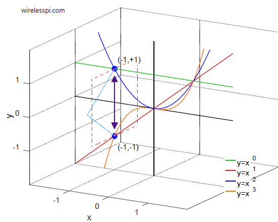
- A complex sinusoid is a fundamental signal that consists of a cosine wave on the real axis and a sine wave on the imaginary axis, as shown below. This is for $z=re^{j\omega}$ when $r=1$.
- Regardless of the signal shape, most signals of practical interest can be considered as a sum of complex sinusoids oscillating at different frequencies, similar to how any point in space can be represented with a combination of x, y and z components, or different colours can be made from the participation of just three basic colours: Red, Green and Blue (a demo for the sinusoids forming a signal is shown here).
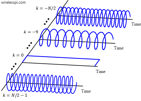
- A set of $N$ orthogonal complex sinusoids is shown below.
- A continuum of such frequencies defines our frequency axis $\omega$ that is employed in DTFT of Eq (\ref{equation-fourier-transform}) above.

Causality
Similar to the DFT, the z-Transform can be thought of as constructing a signal in time domain through complex sinusoids with unit magnitude as well as complex sinusoids scaled by a factor $\neq 1$.
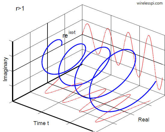
When this factor $r \neq 1$, there are two possibilities. Either $r >1$ (outside the unit circle) or $r<1$ (inside the unit circle).
The complex sinusoids with such magnitude scaling are shown in the figures below. Since $z=re^{j\omega}$ and $r>1$, the magnitude keeps increasing with time for $z^n$ ($n$ is substituted by $t$ for ease of exposition). See the cosine and sine waves growing with time.

On the other hand, the magnitude decays with time for $z^n$ as $r<1$. See the cosine and sine waves diminishing with time.

All the points on the complex z-plane indicate numbers $z$ that (as a function of time) come together to form our signal. Since $z=re^{j\omega}$ and a negative power is used in the definition of z-Transform, we have
\begin{equation}\label{equation-z-general}
z^{-n} = r^{-n} e^{-j\omega n}
\end{equation}
This will have a different impact in case of causal and non-causal impulse responses.
Causal Systems
Causal systems have impulse responses that exist only for $n \ge 0$. For positive $n$, Eq (\ref{equation-z-general}) becomes
\begin{equation}\label{equation-z-causal}
z^{-n} = r^{-n} e^{-j\omega n} = \frac{1}{r^n}e^{-j\omega n}
\end{equation}
Clearly, all signals have a region of convergence when the complex signals decay with time.
- The magnitude is determined by the part involving $r$ because $|e^{-j\omega n}|=1$.
- Since $|r|^n$ appears in the denominator, that happens for $|z|=|r|>1$ here as shown in the figure below.
- For a general case where the outermost pole is $a$, the region of convergence is $|z|=|r|>|a|$. This is because from Eq (\ref{equation-z-causal}), we have
\[
a^n\cdot z^{-n} = a^n\cdot r^{-n} e^{-j\omega n} = \left(\frac{a}{r}\right)^{n} e^{-j\omega n}
\]For all $r$ greater than $|a|$, this sequence converges to zero with time $n$.

In the above figure, the direction of rotations should be clockwise due to negative frequency in $e^{-j\omega n}$ but that is ignored for simplicity.
Non-Causal Systems
Non-causal systems are the ones that exist only for $n < 0$. For these negative values of $n$ denoted by $-n$, Eq (\ref{equation-z-general}) becomes \begin{equation}\label{equation-z-non-causal} z^{-(-n)} = r^{n} e^{j\omega n} \end{equation} Again, all signals should have a region of convergence when the complex signals decay with time.
- Since $|r|^n$ appears in the numerator, that happens for $|z|=|r|<1$ here as shown in the figure below.
- For a general case where the innermost pole is $a$, the region of convergence is $|z|=|r|<|a|$. This is because from Eq (\ref{equation-z-non-causal}), we have \[ a^{(-n)}\cdot z^{-(-n)} = a^{(-n)}\cdot r^{n} e^{j\omega n} = \left(\frac{r}{a}\right)^{n} e^{j\omega n} \] For all $r$ lesser than $|a|$, this sequence converges to zero with time $n$.
- A causal system should have a region of convergence outside the outermost pole.
- A stable system should have the unit circle in its region of convergence.
- Therefore, a causal and stable system should have all poles inside the unit circle.

Stability
With causality established above, it is straightforward to find the stability condition for a system. The system output is determined not by z-Transform but by convolution between the impulse response $h[n]$ and input signal $x[n]$. For a stable system, this convolution output should be finite.
\[
\left|\sum _n h[n]\cdot x[m-n]\right| \le \sum _n \left|h[n]\right|\cdot \left|x[m-n]\right| ~~ \text{is finite}
\]
For a bounded input $x[n]$ that stays lesser than a certain value, the impulse response $h[n]$ should not be growing without bound so that it should produce a bounded output after convolution.
\[
\sum _n |h[n]| ~~ \text{is finite}
\]
Both the causal and non-causal scenarios above involve the role of $r$ for convergence. However, the above expression only focuses on the impulse response samples without $r$ that happens on the unit circle $z=1\cdot e^{j\omega}$ because
\[
|h[n]\cdot 1\cdot e^{-j \omega n}| = |h[n]|
\]
We conclude that the unit circle must be included in the region of convergence for a system to be stable.
Condition for Causal and Stable Systems
The condition for both causality and stability can now be derived as follows.