Gardner Timing Error Detector: A Non-Data-Aided Version of Zero-Crossing Timing Error Detectors

Timing synchronization plays the role of the heart of a digital communication system. We have already seen how a timing locked loop, commonly known as symbol timing PLL, works where I explained the intuition behind the maximum likelihood Timing Error Detector (TED). A simplified version of maximum likelihood TED, known as Early-Late Timing Error Detector, was also covered before. Today we discuss a different timing synchronization philosophy that is based on zero-crossing principle. It is commonly known as Gardner timing recovery.

Background

Before we start this topic, I recommend that you read about Pulse Amplitude Modulation (PAM) for an introduction to digital systems, the framework in which timing synchronization algorithms are described here. The notations for the main parameters are the following.

• Sample time (inverse of sample rate): $T_S$
• Symbol time (inverse of symbol rate): $T_M$
• Data symbols: $a[m]$
• Timing error: $\epsilon _\Delta$
• Timing error estimate: $\hat \epsilon _\Delta$

The samples at the matched filter output in a Pulse Amplitude Modulated (PAM) system are denoted by
\begin{equation*}
\cdots, z((n-2)T_S), z((n-1)T_S), z(nT_S), z((n+1)T_S), z((n+2)T_S), \cdots
\end{equation*}

where $T_S$ is the sampling time and the oversampling factor is 2. The question is: How do we know which sample corresponds to the symbol peak? At the startup time of the Rx, all we have is a series of samples spaced by half-symbol period $T_M/2$ where $T_M$ is the symbol time. Depending on the actual $\epsilon_\Delta$, we could have
\begin{align*}
z((n-2)T_S) ~&\rightarrow~ z((m-1)T_M+\hat \epsilon_\Delta) \quad \text{Symbol Peak}\\
z((n-1)T_S) ~&\rightarrow~ z(mT_M-\frac{T_M}{2}+\hat \epsilon_\Delta) \\
z(nT_S) ~&\rightarrow~ z(mT_M+\hat \epsilon_\Delta) \quad \text{Symbol Peak} \\
z((n+1)T_S) ~&\rightarrow~ z(mT_M+\frac{T_M}{2}+\hat \epsilon_\Delta) \\
z((n+2)T_S) ~&\rightarrow~ z((m+1)T_M+\hat \epsilon_\Delta) \quad \text{Symbol Peak}
\end{align*}

or we could have either $z((n-1)T_S)$ or $z((n+1)T_S)$ correspond to the symbol peak with other samples identified around accordingly. This is because frame synchronization can take us to the correct symbol level only, not the sample.

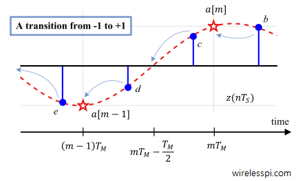
To answer this question, consider the figure below with samples denoted as $b$, $c$, $d$ and $e$.

Applying the early-late equation for three TED samples $b$, $c$ and $d$,
\begin{equation*}
e_D[m] = c\cdot (b-d) > 0
\end{equation*}

However, if we had identified the three TED samples as $c$, $d$ and $e$, then
\begin{equation}\label{eqTimingSyncELTEDexample}
e_D[m] = d\cdot (c-e)
\end{equation}

Since $c-e$ $>$ $0$ and $d$ is negative,
\begin{equation*}
e_D[m] = d \cdot(c-e) < 0 \end{equation*} Instead of $\hat \epsilon_\Delta<\epsilon_\Delta$, the early-late TED then would treat this as a case of late sampling $\hat \epsilon_\Delta>\epsilon_\Delta$ (and hence the negative output in the above expression). The TLL would have brought the sampling instant earlier until the middle sample $d$ reached the instant $(m-1)T_M$ and hence identified as $z((m-1)T_M)$. The left and right samples, namely $e$ and $c$, approach zero in the meanwhile, as illustrated by the figure above.

Towards Zero Crossings

An alternative strategy is a zero crossing timing error detector where the algorithm targets the zero crossings of the waveform. This is done by negating the slope. So let us find out what happens with negating the slope in an early-late expression, for which we again consider the same samples $c$, $d$ and $e$ considered above in Eq (\ref{eqTimingSyncELTEDexample}) with respect to the last figure above.
\begin{align*}
e_D[m] = d\cdot\big\{-(c-e)\big\} = d\cdot (e-c)
\end{align*}

Since $d$ is negative while $e-c$ is also negative,
\begin{equation*}
d \cdot(e-c) > 0
\end{equation*}

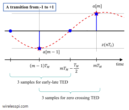
Thus, the sampling instant will be pushed forward until the middle sample $d$ reaches $mT_M-T_M/2$. Then, the left neighbouring sample $e$ will coincide with symbol $a[m-1]$ while the right neighbouring sample $c$ will coincide with $a[m]$. In this game of $3$ samples, the middle sample approaches the zero crossing. This is the philosophy of the zero crossing TEDs.

The converging locations of zero crossing TED as well as early-late TED for the above example are shown in the figure below. Notice that if we had chosen samples $b$, $c$ and $d$ in a zero crossing TED, the middle sample again would have converged towards zero.

From the above analysis, we can form a timing error detector as

This non-data-aided version is called the Gardner Timing Error Detector (TED) due to its inventor F. M. Gardner. Its data-aided and decision-directed versions are commonly known as Zero Crossing Timing Error Detector (TED). By using the data symbols $a[m-1]$ and $a[m]$ in place of $z((m-1)T_M+\hat \epsilon_\Delta)$ and $z(mT_M+\hat \epsilon_\Delta)$, respectively, we get the data-aided variant.
\begin{equation}\label{eqTimingSyncZCTEDDA}
e_D[m] = z\left(mT_M-\frac{T_M}{2}+\hat \epsilon_\Delta\right)\bigg\{a[m-1] – a[m]\bigg\}
\end{equation}

On the same note, a decision-directed form can be created as
\begin{equation}\label{eqTimingSyncZCTEDDD}
e_D[m] = z\left(mT_M-\frac{T_M}{2}+\hat \epsilon_\Delta\right)\bigg\{\hat a[m-1] – \hat a[m]\bigg\}
\end{equation}

where the symbol decision $\hat a[m]$ for a binary PAM case is
\begin{equation*}
\hat a[m] = A \times \text{sign} \Big\{ z(mT_M+\hat \epsilon_\Delta)\Big\}
\end{equation*}

Like derivative and early-late TEDs, a zero crossing approach also depends on balancing the magnitudes of two samples taken midway from either side of the symbol. Consequently, its performance also suffers when the excess bandwidth $\alpha$ is small. See this article for an intuitive explanation of how excess bandwidth impacts the performance of timing synchronization.

Gardner TED is based on the ideas from a wave difference method and a digital Data Transition Tracking Loop (DTTL) (used as a symbol synchronizer in the telemetry Rx of the Mariner Mars 1969 mission.

Receiver Structure

The Rx structure for a zero crossing or Gardner TED is quite similar to that for early-late TED and is drawn in the figure below for a decision-directed setting (click on the image to enlarge it).

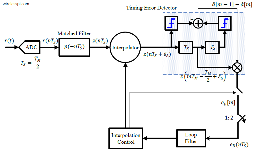
The Rx signal $r(t)$ is sampled at a rate of $F_S=2/T_M$, or $T_S=T_M/2$, to generate $r(nT_S)$ at $L=2$ samples/symbol. Next, the sampled signal $r(nT_S)$ is matched filtered at the same rate with its output being $z(nT_S)$. Under the command of an interpolation control block, an interpolator resamples these matched filter outputs at instants $\hat \epsilon_\Delta$ to produce $z(nT_S+\hat \epsilon_\Delta)$. Since this system runs at a rate of 2 samples/symbol, the delay block $T_S$ (that represents a delay of 1 sample) supplies the samples at half a symbol duration, i.e., $z(mT_M-T_M/2+\hat \epsilon_\Delta)$.

The interpolation control block also identifies the time instants $(m-1)T_M$ and $mT_M$ at which the outputs $\hat a[m-1]$ and $\hat a[m]$ are taken out of the decision block and the error signal $e_D[m]$ is formed once per symbol. In the case of Gardner TED, the matched filter outputs $z((m-1)T_M+\hat \epsilon_\Delta)$ and $z(mT_M+\hat \epsilon_\Delta)$ are directly used instead of $\hat a[m-1]$ and $\hat a[m]$ in forming the TED output. This signal $e_D[m]$ is then upsampled by $2$ to create $e_D(nT_S)$ that then matches the sample rate $F_S$ of the loop filter and the interpolation control.

Example

Now we simulate a Gardner TED for the same set of parameters as for a derivative TED here except $L$ which is $2$ in this case, i.e.,
\begin{align*}
\text{Modulation} \quad \rightarrow&\quad 2-\text{PAM}, \\ L \quad =& \quad 2 ~\text{samples/symbol}, \\ \alpha \quad =& \quad 0.4, \\
B_n T_M\quad =& \quad 1/200, \\ \zeta \quad =& \quad 1/\sqrt{2}, \\ \epsilon_\Delta \quad =& \quad 0.25 T_M
\end{align*}

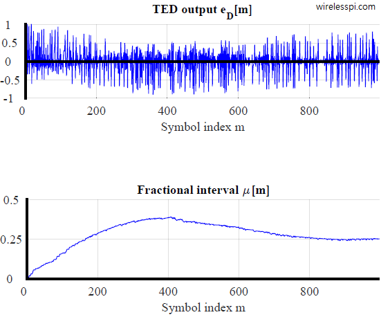
Again, the PI loop filter coefficients are computed from Eq (4) of the PLL article where $K_0$ is unity while a simple routine is used to compute the derivative of the mean curve at $\epsilon_\Delta=0$ for $K_D$. The output error signal $e_D[m]$ for a Gardner TED is shown in the figure below where the estimate of the timing offset $\epsilon_\Delta=0.25T_M$ is seen converging to its true value. We call this estimate as a fractional interval $\mu[m]$. The TLL is seen to converge in approximately $800$ symbols.

Finally, the zero crossing TED for a QAM scheme is given by the sum of inphase and quadrature parts. For example, from Eq (\ref{eqTimingSyncZCTEDDA}), the data-aided version can be written as
\begin{equation*}
\begin{aligned}
e_D[m] &= z_I\left(mT_M-\frac{T_M}{2}+\hat \epsilon_\Delta\right)\bigg\{a_I[m-1] – a_I[m]\bigg\} + \\
&\hspace{.3in}z_Q\left(mT_M-\frac{T_M}{2}+\hat \epsilon_\Delta\right)\bigg\{a_Q[m-1] – a_Q[m]\bigg\}
\end{aligned}
\end{equation*}

Carrier Independent Operation

One of the reasons for popularity of Gardner TED was the belief that its operation is independent of the carrier phase as well as a small frequency offset. Many sources still cite the Gardner TED as having an extra feature of rotationally invariant (carrier independent operation) and hence very suitable for timing acquisition when a significant carrier phase offset and possibly a small carrier frequency offset is present in the Rx signal.

As it turns out, this carrier independent operation is not exclusive to the Gardner TED. In fact, this is a feature of the non-data-aided fashion in which the TED processes the Rx samples. For passband modulation schemes, the Gardner TED is given from complex samples by the inphase part of a conjugate product instead of a simple product.
\begin{equation*}
e_D[m] = \bigg[z\left(mT_M-\frac{T_M}{2}+\hat \epsilon_\Delta\right)\bigg\{z^*\left((m-1)T_M+\hat \epsilon_\Delta\right) – z^*\left(mT_M+\hat \epsilon_\Delta\right)\bigg\}\bigg]_I
\end{equation*}

From the definition of a complex conjugate $V^*$, we know that
\begin{align*}
\begin{aligned}
|V^*| &= |V| \\
\measuredangle V^* &= – \measuredangle V
\end{aligned}
\end{align*}

Consequently, the phase of the middle sample is canceled by the common phase of the two samples in the brackets above. However, the non-data-aided version of early-late TED exhibits exactly the same property for complex samples.
\begin{equation*}
e_D[m] = \bigg[z(mT_M+\hat \epsilon_\Delta) \left\{z^*\left(mT_M+\frac{T_M}{2}+\hat \epsilon_\Delta\right) – z^*\left(mT_M-\frac{T_M}{2}+\hat \epsilon_\Delta\right)\right\}\bigg]_I
\end{equation*}

In terms of complex signals, $\exp\left(j\theta\right)$ is the phase rotation of the middle sample while $\exp\left(-j\theta\right)$ can be taken as common from the terms in the brackets.

In conclusion, as long as there is a conjugate product being taken between the complex samples having the same phase rotation, the TED is essentially carrier independent and Gardner TED is not unique in this regard. Having said that, the presence of a rotating phase in the constellation can perturb the timing error detectors to some extent in terms of the jitter and acquisition time.

Final Remarks

There are some final comments in regards to this discussion as follows.

• There has been a long standing confusion in synchronization community regarding the non-data-aided early-late and Gardner timing error detectors that has been clarified here.
• For an example of a timing recovery system that can be implemented after carrier recovery at 1 sample/symbol, see the Mueller and Muller algorithm.
• Feedforward techniques that do not require a PLL are also possible such as digital filter and square timing synchronization.