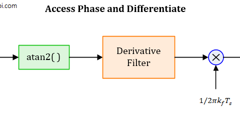
In an article on Phase Locked Loop (PLL) for symbol timing recovery, we described an intuitive view of a maximum likelihood Timing Error Detector (TED). We saw that the timing matched filter is constructed by computing the derivative of the matched filter and consequently its output is the derivative of the input signal. Naturally, this output is more fine-grained and hence accurate when the number of samples/symbol $L$ is large. Here, $L$ must be several times larger than the minimum limit set by the Nyquist theorem.
However, in most applications, reducing the complexity of the timing locked loop is far more desirable than achieving the gains from the increased granularity. Instead of having a vastly oversampled Rx signal, a simpler form of a timing error detector is therefore attractive for system design operating at no more than $1$ or $2$ samples/symbol. Due to this reason, there are many approximations to the maximum likelihood timing error detector that have been derived over the years. Some of those new TEDs were invented in an ad-hoc fashion that turned out to be just another of its approximations. Early-late timing synchronizer is built on one such approximation.
Simplifying the Derivative
Carrying on from the timing locked loop, assume that the Rx signal is sampled at $L=2$ samples/symbol. In this case, the matched filter output, denoted by $z(nT_S)$, has every other sample that is a candidate of the symbol decision, i.e., $m=2n$. To keep the indexing in terms of symbols rather than samples, a better notation is to use $mT_M$ for the main sample as before and use $\pm T_M/2$ for the intermediate sample.
\begin{align*}
&\cdots, z\left((m-1)T_M+\hat \varepsilon_\Delta\right), z\left(mT_M-\frac{T_M}{2}+\hat \varepsilon_\Delta\right),z(mT_M+\hat \varepsilon_\Delta),\\
&\hspace{1.8in}z\left(mT_M+\frac{T_M}{2}+\hat \varepsilon_\Delta\right),z\left((m+1)T_M+\hat \varepsilon_\Delta\right),\cdots
\end{align*}
In the above time series of the matched filter output,
- $z((m-1)T_M+\hat \varepsilon_\Delta)$ is a candidate for symbol decision for symbol $m-1$,
- $z(mT_M-T_M/2+\hat \varepsilon_\Delta)$ is an intermediate sample only useful for TED operation,
- $z(mT_M+\hat \varepsilon_\Delta)$ is a candidate for symbol decision for symbol $m$,
- $z(mT_M+T_M/2+\hat \varepsilon_\Delta)$ is an intermediate sample only useful for TED operation, and
- $z((m+1)T_M+\hat \varepsilon_\Delta)$ is a candidate for symbol decision for symbol $m+1$.
Now recall that a popular approximation to compute the derivative of a waveform at a time $n$ is the first central difference filter
\begin{equation*}
h[n] = \left\{+1,0,-1\right\}
\end{equation*}
where the scaling factor $1/2$ is removed for simplification. A reduced complexity solution is to just apply this filter to the matched filter output for finding its approximate slope. For this purpose, concentrate on the matched filter output $z(mT_M)$ and the two samples around it, that is to say
\begin{equation*}
z\left(mT_M-\frac{T_M}{2}+\hat \varepsilon_\Delta\right),z(mT_M+\hat \varepsilon_\Delta),z\left(mT_M+\frac{T_M}{2}+\hat \varepsilon_\Delta\right)
\end{equation*}
These samples are drawn in the figure below, where the slope is being computed at time $mT_M+\hat \varepsilon_\Delta$. In this scenario,
- the symbol candidate $z(mT_M+\hat \varepsilon_\Delta)$ corresponds to the symbol $a[m]$ (sometimes referred to as ‘prompt’),
- $z(mT_M-T_M/2+\hat \varepsilon_\Delta)$ is an early sample, and
- $z(mT_M+T_M/2+\hat \varepsilon_\Delta)$ is a late sample.

These early and late samples, namely $z(mT_M-T_M/2+\hat \varepsilon_\Delta)$ and $z(mT_M+T_M/2+\hat \varepsilon_\Delta)$ respectively, can be employed for computing the derivative because they overlap with the coefficients $-1$ and $+1$ of $h[-n]$ during the convolution process, as shown in the figure above (remember one of the signals, $h[n]$ here, is reversed during convolution). A seesaw perspective explained here further clarifies how an early-late TED tries to balance the input samples.
A timing error detector operates at the output of the interpolator. That is, a TED input is the samples interpolated at certain locations depending on $\hat \varepsilon_\Delta$. Thus, a non-data-aided Early-Late Timing Error Detector (TED) can be constructed by replacing the derivative term $\smash{\overset{\centerdot}{z}(mT_M+\hat \varepsilon_\Delta))}$ in the maximum likelihood TED as
\begin{equation}\label{eqTimingSyncELTEDNDA}
e_D[m] = z(mT_M+\hat \varepsilon_\Delta) \left\{z\left(mT_M+\frac{T_M}{2}+\hat \varepsilon_\Delta\right) – z\left(mT_M-\frac{T_M}{2}+\hat \varepsilon_\Delta\right)\right\}
\end{equation}
Naturally, its data-aided version can also be made by using the known symbol $a[m]$ in place of $z(mT_M+\hat \varepsilon_\Delta)$.
\begin{equation}\label{eqTimingSyncELTEDDA}
e_D[m] = a[m] \left\{z\left(mT_M+\frac{T_M}{2}+\hat \varepsilon_\Delta\right) – z\left(mT_M-\frac{T_M}{2}+\hat \varepsilon_\Delta\right)\right\}
\end{equation}
On the same note, a decision-directed early-late TED can be created as
\begin{equation}\label{eqTimingSyncELTEDDD}
e_D[m] = \hat a[m] \left\{z\left(mT_M+\frac{T_M}{2}+\hat \varepsilon_\Delta\right) – z\left(mT_M-\frac{T_M}{2}+\hat \varepsilon_\Delta\right)\right\}
\end{equation}
Rx Structure for Early-Late Synchronizer
We now look into the Rx structure for an early-late TED for which a block diagram in a decision-directed setting is shown in the figure below (click to enlarge). The Rx signal $r(t)$ is sampled at a rate of $F_S=2/T_M$, or $T_S=T_M/2$, to generate $r(nT_S)$ at $L=2$ samples/symbol. Next, the sampled signal $r(nT_S)$ is matched filtered at the same rate with its output being $z(nT_S)$.
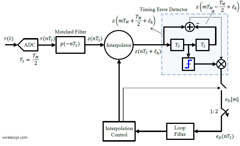
Under the command of an interpolation control block, an interpolator resamples these matched filter outputs at instants $\hat \varepsilon_\Delta$ to produce $z(nT_S+\hat \varepsilon_\Delta)$. Since this system runs at a rate of $2$ samples/symbol, the delay block $T_S$ (that represents a delay of $1$ sample) supplies the samples at half a symbol duration, i.e., $z(mT_M-T_M/2+\hat \varepsilon_\Delta)$ and $z(mT_M+T_M/2+\hat \varepsilon_\Delta)$.
The interpolation control block also identifies the time instants $mT_M$ at which the output $\hat a[m]$ is taken out of the decision block and the error signal $e_D[m]$ is formed once per symbol according to Eq \eqref{eqTimingSyncELTEDDD}. This is because the decisions and hence the early-late TED output should be constructed only every other sample, not each sample. In the case of non-data-aided operation, the matched filter output $z(mT_M+\hat \varepsilon_\Delta)$ is directly used instead of $\hat a[m]$ in forming the TED output. This signal $e_D[m]$ is then upsampled by $2$ to create $e_D(nT_S)$ which matches the sample rate $F_S$ of the loop filter and the interpolation control.
Alternative Forms of Early-Late Timing Error Detectors
Another more familiar form of an early-late TED can now be understood starting from the fundamental relation $|z(nT_S|^2$ employed for timing recovery. Simply apply the definition of a derivative in discrete domain to get
\begin{equation*}
\frac{\partial}{\partial \hat \varepsilon_\Delta} \Big|z(mT_M+\hat \varepsilon_\Delta)\Big|^2 \approx \frac{|z(mT_M+\hat \varepsilon_\Delta+\delta)|^2 – |z(mT_M+\hat \varepsilon_\Delta-\delta)|^2}{2\delta}
\end{equation*}
where $\delta$ is a fraction of the symbol time. Ignoring the constant $2\delta$ in the denominator, an error signal can be formed as
\begin{equation*}
e_D[m] = |z(mT_M+\hat \varepsilon_\Delta+\delta)|^2 – |z(mT_M+\hat \varepsilon_\Delta-\delta)|^2
\end{equation*}
Another version of this TED can be formed as
\begin{equation*}
e_D[m] = |z(mT_M+\hat \varepsilon_\Delta+\delta)| – |z(mT_M+\hat \varepsilon_\Delta-\delta)|
\end{equation*}
It is obvious that the former version is called the square law early-late TED while the latter is called the absolute value early-late TED.
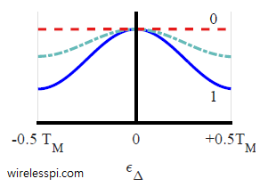
These are known as non-coherent version of the early-late TED. To understand their operation, consider the figure below that plots an average squared trajectory of a binary PAM sequence filtered with a Raised Cosine filter for three different excess bandwidths $\alpha$ $= 0, 0.5$ and $1$. Notice that the average value for $\alpha=0$ is flat with no dependence on the timing error. Therefore, it provides no relevant information for timing synchronization. On the other hand, $\alpha=0.5$ and $\alpha=1$ provide suitable timing information due to the dependence of their average curves on the timing error. See this article for a more detailed explanation of the impact of excess bandwidth on timing synchronization.

Clearly, the ‘heavier’ side yields the error sign for subsequent correction like a seesaw. Computing difference in such a manner has the benefit that there is no need to use the matched filter output $z(mT_M+\hat \varepsilon_\Delta)$, or its decision $\hat a[m]$ for the TED output. The difference is zero when both the early and late samples reach the same value on the average squared curve, see the figure below. The main disadvantage is the extra sample required at the peak of the matched filter output for detection purpose.

Yet other versions of an early-late TED also exist. One such type of early-late TED is described as
\begin{equation*}
e_D[m] = z(mT_M+\hat \varepsilon_\Delta) \big\{z\left(mT_M+T_S+\hat \varepsilon_\Delta\right) – z\left(mT_M-T_S+\hat \varepsilon_\Delta\right)\big\}
\end{equation*}
where $T_S$ is the sample rate of the system, often chosen as $T_M/4$ for accessing the two sizeable slopes. At a sample rate of $L=4$ samples/symbol, this is relatively an inefficient method emulated from the analog period to implement digital transceivers.
Final Remarks
There are some comments related to the early-late synchronizer as follows.
- Early-late TED has been quite popular for timing recovery applications even before the digital era and shows continued interest during the subsequent evolution towards digital signal processing techniques. It has been widely used for timing recovery applications not only in digital communication systems but in global positioning systems as well.
- It is also reminiscent of the dual-window range gate scheme applied in Distance Measuring Equipment (DME) with an early and a late range gate aligned for pulse arrival.
- You can explore other timing synchronization algorithms too. Some of the feedback techniques are a zero-crossing approach and Mueller and Muller algorithm. Timing can also be recovered through a feedforward method such as digital filter and square timing synchronization.
- There has been a long standing confusion in synchronization community regarding the non-data-aided early-late and Gardner detectors that has been clarified here.
Thank you for explanation.
Is there a way to do time synchronization without knowing the oversampling factor L at the receiver? How can I estimate the oversampling factor?
Oversampling factor at the transmitter and receiver do not have to be the same. So it doesn’t matter what was chosen at the Tx side (as opposed to other parameters like symbol rate, excess bandwidth, etc.). Therefore, at the receiver, the oversampling factor L is your own decision and does not need to be estimated anywhere.
How will it change if i have say 256 samples in one symbol?
If you want to use an early-late bit synchronizer, the signal needs to be downsampled to 2 samples/symbol. Instead of a separate lowpass filter, the downsampling can be incorporated into the matched filter.
Now if you do have 256 samples/symbol coming in, I would recommend using a polyphase matched filter and symbol timing recovery. See the 2001 paper by fred harris and Michael Rice: “Multirate digital filters for symbol timing synchronization in software defined radios”.