The Big Picture of Localization

Digital Signal Processing (DSP) enables us to find the range of a device transmitting a wireless signal with a particular structure under some conditions. To understand how this process works, we need to look at the big picture of a localization process. Localization implies locating the unknown position of a source which can be computed in a straightforward manner if its ranges from some reference nodes can be found.

Various techniques are employed for this purpose, some of which are Received Signal Strength Indicator (RSSI), time of arrival, time difference of arrival and angle of arrival. Phase of arrival is a special case of time of arrival scheme which is extremely accurate due to the high frequency carrier resembling a high resolution clock. This method works even in the absence of synchronization among nodes. Here, I will discuss various arrangements under which finding the range and/or position of the device becomes feasible for time of arrival technique. It is worth noting that since phase is just another manifestation of time, the underlying principles stay the same.

One Way Transmission

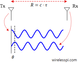
Let us start with a transmitter Tx whose signal is received by a receiver Rx. The electromagnetic signal travelling at a speed of $c=3\cdot 10^8$ m/s takes a finite amount of time $\tau$ to arrive at the Rx. This is shown in the figure below and from basic physics, the range $R$ is given by
\begin{equation*}
R = c\tau
\end{equation*}

This propagation delay $\tau$ is our main target for ranging purpose. However, since each node starts at a random time, there is a clock offset between its time as compared to the real time. At an arbitrary real time 0, the time offset of the Tx is $\theta_{\text{Tx}}$ while that of of the Rx is $\theta_{\text{Rx}}$.
\begin{equation*}
\begin{aligned}
T_{\text{Tx}} &= t + \theta_{\text{Tx}} \\
T_{\text{Rx}} &= t + \theta_{\text{Rx}}
\end{aligned}
\end{equation*}
where $t$ is the real time. What happens at the Rx side if we implement one way transmission in which the Tx emits the wave at real time $t_{\text{Tx}}$ received by the Rx at real time $t_{\text{Rx}}$?
\begin{equation}\label{eq1WayTransmission1}
t_{\text{Rx}}-\theta_{\text{Rx}} = t_{\text{Tx}} – \theta_{\text{Tx}} + \tau
\end{equation}
We can reduce three unknowns to two by combining the individual phase offsets into one entity $\theta$.
\begin{equation*}
\theta = \theta_{\text{Rx}} – \theta_{\text{Tx}}
\end{equation*}
Then, Eq (\ref{eq1WayTransmission1}) can be written as
\begin{equation}\label{eq1WayTransmission2}
t_{\text{Rx}} = t_{\text{Tx}} + \theta + \tau
\end{equation}
This equation still has two unknowns $\theta$ and $\tau$. As a side remark, notice in the above figure that unique range can only be found if the distance between the Tx and Rx is within one wavelength only. At high carrier frequencies, e.g., 2.4 GHz where the wavelength is just 12.5 cm, the phase of arrival method seems impractical due to $2\pi$ phase ambiguity. Nevertheless, transmissions at multiple carrier frequencies solve this range ambiguity problem in frequency domain.

To summarize, we get only one equation from this procedure and hence it becomes impossible to separate the phase offset $\theta$ from propagation delay $\tau$ in time domain. There are several ways in which one or more extra equations can be provided to this system for range determination.

Solution 1: Synchronization

We can synchronize the two nodes which implies that $\theta$ becomes zero. From Eq (\ref{eq1WayTransmission2}), we can write

\begin{equation*}
t_{\text{Rx}} = t_{\text{Tx}} + \tau
\end{equation*}

This leaves us with one equation and one unknown, i.e., delay $\tau$. Synchronizing the Tx and Rx is not straightforward however and consumes resources either in terms of cost or computations.

Solution 2: Back and Forth Transmission

Realizing that two unknowns can be solved through a system of two equations, we can provide an extra independent equation through back and forth transmission between the Tx and Rx. The original timestamps or phases at the Tx and Rx during the forward transmission can now be denoted with the subscript 1 while the subscript 2 can be used for the backward transmission from the Rx to the Tx.
\begin{equation*}
\begin{aligned}
t_{Rx,1} &= t_{Tx,1} + \theta + \tau \\
t_{Tx,2} &= t_{Rx,2}~ – \theta + \tau
\end{aligned}
\end{equation*}

In this scenario, the phase offset $\theta$ appears with a negative sign in the second equation because timing or phase measurement is done at the transmitter (known as the initiator here). If you are unsure about this sign change, start with the basic definitions of phase offsets mentioned before. Now we have two equations that can solve the two unknowns $\theta$ and $\tau$. Multiple carrier phases can also be utilized for ranging purpose in multipath channels.

Solution 3: Motion

The above system of equations provides a second independent equation in terms of a negative sign with the phase offset $\theta$ where the first equation contains $+1$ as the coefficient for both $\theta$ and $\tau$. This concept can be generalized to provide a second equation to this system with any other coefficient to either $\theta$ or $\tau$. This is difficult to accomplish this with the phase offset $\theta$. On the other hand, we can always move one node around that changes the coefficient that appears with $\tau$ without affecting the phase offset $\theta$.

For example, if the Rx moves twice as far as compared to the original range, we get

\begin{equation*}
\begin{aligned}
t_{Rx,1} &= t_{Tx,1} + \theta + \tau \\
t_{Rx,2} &= t_{Tx,2} + \theta + 2\tau
\end{aligned}
\end{equation*}

Note that both transmissions in this case are in the same direction from the Tx to the Rx, as opposed to the back and forth solution. A subtle but really important point here is to come up with a strategy to produce a known coefficient for delay $\tau$ which in general is not easy due to $\tau$ itself being unknown. Researchers have come up with several smart algorithms for this purpose, one of which was very well explained by Marcus Müller during a short discussion with me on discuss-gnuradio archive.

From Range to Position

All three solutions above are applicable to a Tx and a Rx only, thus giving us the range between them. To obtain the position of a device, extra equations are needed within this system. For this purpose, we can place extra anchor nodes around the Tx with known positions.

One issue here is that exactly the same number of extra phase offsets appears in the set. To alleviate this problem, these anchor nodes can be synchronized with a common reference which is how a GPS Rx finds its position through a synchronized network of satellites. Assuming perfect synchronization among them, the receiver phase offset $\theta$ is the same for all received satellite signals.

Interestingly, injecting multiple measurements into the system is exactly how the challenging problem of finding the distance between the earth and the sun was solved in the 18th century. Author Y. Harari writes the following lines in ‘The Marriage of Science and Empire’:

Another option is that after the Tx signal is received by all surrounding nodes, one node can respond with a reply message which makes the phase offsets appear with negative signs making the system solvable. This is usually known as ranging through one-way transmission (or blink mode) because target node has to transmit only once.

You might also enjoy reading the article on Frequency Modulated Continuous-Wave (FMCW) radar.

References

[1] OFDM Radar Algorithms in Mobile Communication Networks