In an article on carrier phase based ranging, we saw how phase observations were employed to find the range between two wireless devices. Today we explore how phase can also be used for the purpose of location estimation.
Background
To determine the position of a wireless device, its range needs to be computed from a set of anchor nodes. When these anchors and the device itself are synchronized with each other, the signal propagation time of an electromagnetic wave arriving at these anchors after its emission from a Tx can be employed to calculate the corresponding distances. This is the well known time of arrival problem. With an unsynchronized wireless device, time difference of arrival utilizes the difference in signals propagation durations from the Tx arriving at the receivers.
Phase Difference of arrival (PDoA) is a special case of time difference of arrival. However, for a completely unsynchronized system in which the anchor nodes as well as the wireless device have their own free-running clocks, differential readings at these anchor nodes can be employed to estimate the target position. Differential Phase Difference of arrival (DPDoA) is a special case of differential time difference of arrival in which the same principle is used with phase measurements.
Set Up
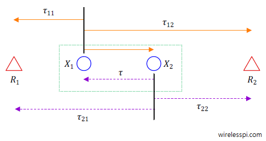
To understand this method, we consider a one-dimensional setup so that there are two receive-only anchor nodes recording their own phase measurements from the signal exchange between a maser and a slave node in a two-way scenario. This is drawn in the figure below where the parameters $\tau_{11}$, $\tau_{12}$, $\tau_{21}$ and $\tau_{22}$ denote the time delays $\tau_{ij}$ from a node $i$ to a node $j$.

The node $X_1$ emits a signal in a channel defined for a certain band while the node $X_2$ replies with an automatic acknowledgement packet (AACK) after a certain delay.
This delay $T_{\text{turnaround}}$ in a two-way system is either known beforehand through empirical means or calibrated before the experiments. However, for a DPDoA setup, this cancels out in the final result as we see now.
The Algorithm
Since it is easier to grasp the ranging and synchronization parameter estimation through time based measurements and phase is just another manifestation of time with a frequency scaling, we present the relevant equations in terms of time steps and later convert the results into phase measurements in a straightforward manner. The $n^{\text{th}}$ readings at anchor nodes $R_1$ and $R_2$ are given as
\begin{align*}
\delta T_{1\rightarrow 1}[n] &= \tau_{11} + \phi_{R_1} \\
\delta T_{1\rightarrow 2}[n] &= \tau_{12} + \phi_{R_2} \\
\delta T_{2\rightarrow 1}[n] &= \tau_{21} + \phi_{R_1} + T_{\text{turnaround}}\\
\delta T_{2\rightarrow 2}[n] &= \tau_{22} + \phi_{R_2} + T_{\text{turnaround}}
\end{align*}
Subtracting the corresponding equations at one Rx yields
\begin{align*}
\Upsilon_1[n] &= \delta T_{2\rightarrow 1}[n]-\delta T_{1\rightarrow 1}[n] = \tau + T_{\text{turnaround}}\\
\Upsilon_2[n] &= \delta T_{2\rightarrow 2}[n]-\delta T_{1\rightarrow 2}[n] = -\tau + T_{\text{turnaround}}
\end{align*}
where the relations $\tau$ $=$ $\tau_{21}-\tau_{11}$ $=$ $\tau_{12}-\tau_{22}$ are evident from the above figure. From here, the delay $\tau$ can be found as
\begin{align*}
\Upsilon[n] &= \Upsilon_1[n] – \Upsilon_2[n] \\
&= \delta T_{2\rightarrow 1}[n]-\delta T_{1\rightarrow 1}[n] – \delta T_{2\rightarrow 2}[n]+\delta T_{1\rightarrow 2}[n] = 2\tau
\end{align*}
Going towards the phase measurements now, we can write the phase equations for the $k^{\text{th}}$ subchannel corresponding to the above timestamps as follows.
\begin{equation*}
\Upsilon[k] = \delta \phi_{2\rightarrow 1}[k]-\delta \phi_{1\rightarrow 1}[k] – \delta \phi_{2\rightarrow 2}[k]+\delta \phi_{1\rightarrow 2}[k]
\end{equation*}
As described earlier, this set of phase measurements must be collected for each subchannel $k$. Once this is done, the position of the device can be easily computed by stitching them together.