Indoor positioning is one of the core technologies behind the idea of Internet of Things (IoT). Some of the use cases are asset tracking and management, factory automation systems, virtual and augmented reality applications, social media relevance and precision marketing in shopping malls. Distances between wireless devices can be determined through various ranging techniques that were introduced in the big picture of localization. Among the candidates, phase based ranging is a low-cost and accurate method that can be implemented on cheap hardware and deployed in real scenarios with relative ease (even in the absence of synchronization among nodes). In this article, the phase slope method will be explained in detail.
Background
The bane of almost all indoor localization techniques is the signal echoes arriving at the Rx from multiple paths. This multipath is a more serious challenge for localization than communication because we can always employ an equalizer to compensate for the channel impact in the latter case. In the former case, however, late arriving echoes significantly alter
- the received amplitude for received signal strength measurements,
- spread the peak of the correlation for time of flight, and
- change the phase of each carrier through vector summation.
To solve the challenge a phase based ranging system must overcome in a multipath scenario, we need to understand the effect of this multipath channel on a time based ranging system.
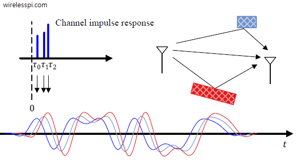
In this setup, several echoes of the ranging signal are arriving at the Rx and distorting the original pulse shape which makes it difficult to identify the earliest arriving pulse for ranging purpose. The expression for the impulse response of a short term time-invariant channel is given as
\begin{equation}\label{eqMultipath}
h(t) = \sum_{i=0}^{L-1} \rho_i\cdot \delta (t-\tau_i)
\end{equation}
where $L$ is the total number of multiple paths while $\rho_i$ and $\tau_i$ are the amplitude and delay of $i^{\text{th}}$ path, respectively.
To zoom into this cumulative outcome, we first delve into the role of bandwidth in a range measuring equipment because it determines the pulse rise time of our timing markers. This involves not only Tx and Rx filtering but also the frequency response of the frontend filters as well as of the multipath channel. For the sake of simplicity, we confine our discussion to the Tx and Rx filters.
Role of Bandwidth
As an example, the spectrum and time domain waveform for a Raised Cosine pulse shape that is most commonly used in digital communication systems are drawn in the figure below for rise time $T_R$ and excess bandwidth $\alpha=0.5$.

Observe that there is an inverse relationship between the pulse rise time and the bandwidth as
\begin{equation*}
B = \frac{1+\alpha}{2T_R}
\end{equation*}
As the pulse gets narrow in time domain (a small $T_R$), the bandwidth $B$ expands in an inverse proportion.
As an approximation to derive a rule of thumb, we put $\alpha=0$ that corresponds to a rectangular spectrum.
\begin{equation*}
B = \frac{1}{2T_R}
\end{equation*}
For instance, a range resolution of under a meter requires a timing resolution of $1\text{m}/(3\cdot 10^8 \text{m/s})$ $=$ $3.33$ ns. The required bandwidth then is given by
\begin{equation}\label{eqUWB}
B = \frac{1}{3.33~\text{ns}} = 300~ \text{MHz}
\end{equation}
One implication of this relation is that for a low bandwidth signal, the pulse rise time $T_R$ is quite long which in isolation is not a problem. However, this becomes a significant challenge in a multipath channel where multipath components arrive at the Rx after being reflected from the nearby surfaces. This is shown in the figure below for a $3$-path channel whose impulse response is also drawn.

In indoor applications, a distance resolution of 1 m is often desired which translates to a time resolution of $3.33$ ns as seen above. However, the indoor paths can differ by several meters which implies that they can arrive as late as a few tens of nanoseconds. Let us see how it affects the range estimation process.
There are different techniques to detect the signal arrival time, some of which are transmitting a narrow pulse or achieve pulse compression through spreading the spectrum with the help of a discrete sequence or an increasing/decreasing chirp. In any case, in time based ranging systems, a cross-correlation between the received signal $r(t)$ and the expected signal $s(t)$ is computed at the Rx to determine the arrival time. This cross-correlation is defined as
\begin{equation*}
y[n] = \sum \limits _{m = -\infty} ^{\infty} r[m] s^*[m-n]
\end{equation*}
The index $n$ determines the correlation output which marks a narrow peak in time. At $n=0$, i.e., when the received signal and the stored signal are in complete sync with each other in a single path environment, the output has a maximum value that is significantly larger than other values of $n$ due to the good correlation properties of the ranging signal.
In a multipath channel where the delay of the second arriving echo is on the order of the pulse rise time which is the case frequently encountered in indoor environments, their natural summation at the Rx antenna distorts the correlation output and makes it deviate from a single and clearly defined peak. This is shown in the figure below in terms of distance (and not time) where the channel consists of three paths:
- a direct path with a length of $9$ m,
- a second path with a length of $13$ m, and
- a third path with a length of $15$ m.
It is clear from the figure that a high bandwidth pulse, which is narrow in time domain, has a higher resolution in time domain and all three paths can be differentiated in this case. On the other hand, the low bandwidth pulse has a low resolution in time and the summation of arriving echoes results in the peak moved to $15$ m. This induces a penalty of $6$ m in range estimation.

Phase Slope Method in a Single Path Environment
To combat interference and multipath in indoor channels, a number of difference continuous waves can be used and their results can be stitched together to form a precise range estimate. To understand this process, assume that we are operating in the $2.4$ GHz ISM band in a channel with a single direct path and utilize the available frequencies from $2.4$ GHz to $2.48$ GHz for a total bandwidth of $80$ MHz. This spectrum can be divided into $N=80$ subchannels with a frequency separation $\Delta_\text{F}$ $=$ $1$ MHz between them. The Tx sends a CW at each of these $80$ subchannels during one-way communication while the Rx downconverts and measures the phase for each such frequency. For a single path normalized amplitude environment and subchannel $k$ at carrier frequency $F_k$,
\begin{equation*}
e^{j2\pi F_k t}*\delta (t-\tau) = e^{-j2\pi F_k \tau} e^{j2\pi F_k t}
\end{equation*}
where the phase term can be explicitly taken out (one-way communication implies a factor of $2\pi$ with the phase). After taking the desired number of measurements for a direct path at a distance of $9.9$ m (a delay of $33$ ns), a plot of phase versus frequency is drawn in the figure below in the presence of AWGN only and no multipath. Also shown is a line fit that can be utilized to estimate the true range.
- The original wrapped phase is drawn against frequency in the top figure.
- A phase unwrapping algorithm can be employed to straighten this phase data. This unwrapped phase is plotted in the bottom figure for all subchannels and its slope can be extracted to measure the range, as explained next.

Let us see how the range can be estimated in a 2-way signal exchange scenario now. Similar to Eq (6) here, we can write
\[
\Delta \theta_{\text{frac},F_k} = 2\pi\left(2R\frac{F_k}{c} + \text{constant}\right)
\]
where the constant term arises instead of $n$ as it might not be the same for all frequencies. The time intervals between phase measurements must be constant and same at both nodes. Note that after phase unwrapping, the slope of the curve is still given by
\[
\text{slope} = \frac{4\pi}{c}\cdot R
\]
from which the range can be found as
\[
R = \frac{c}{4\pi} \cdot \text{slope}
\]
This is why it is known as the Phase Slope method. It is relatively costly to implement due to a number of back and forth transmissions (equal to the number of CWs employed) but it is very accurate due to the wider bandwidth employed. Next, we describe how the phase slope method deals with a multipath environment.
Phase Slope Method in a Multipath Environment
We start with the expression in Eq (\ref{eqMultipath}) for a multipath channel impulse response and see the outcome when a continuous wave or a complex sinusoid $e^{j2\pi F_k t}$ at a carrier frequency $F_k$ is injected into the channel. Being a linear time-invariant system, the result is the convolution between the signal and the channel impulse response.
\begin{align*}
r(t) &= e^{j2\pi F_k t} * h(t) = e^{j2\pi F_k t} * \sum_{i=0}^{L-1} \rho_i\cdot \delta (t-\tau_i) \\
&= \sum_{i=0}^{L-1} \rho_i e^{j2\pi F_k (t-\tau_i)} = \sum_{i=0}^{L-1} \rho_i e^{-j2\pi F_k \tau_i} e^{j2\pi F_k t} = a_k e^{j2\pi F_k t}
\end{align*}
where $a_k$ is the complex gain of the $k{\text{th}}$ complex sinusoid at the Rx side that arises from the vector sum of the amplitudes and phases of the arriving echoes.
\begin{equation}\label{eqMultipathSum}
a_k = \sum_{i=0}^{L-1} \rho_i e^{-j2\pi F_k \tau_i}
\end{equation}
We deduce that while each multipath copy of a complex sinusoid arrives with the same frequency $F_k$ but an amplitude $\rho_i$, its phase is also changed by an amount $-2\pi F_k\tau_i$. For example, for a single multipath copy arriving with amplitude $\rho_1$ at $\tau_1$ seconds after the direct path, this phase shift is illustrated in the figure below along with the direct path. The result for several multipath signals can be produced by extending the same concept, i.e., when many of these vectors are added for the same subcarrier frequency $F_k$, we get the channel coefficient for each $F_k$ as a vector sum of the channel taps.

From the above discussion, the phase information does not seem to get preserved. Let us first see how it changes and then draw a similar phase versus frequency plot as in the single path scenario but in a multipath environment. For a two path channel, Eq (\ref{eqMultipathSum}) can be written as
\begin{align*}
a_k = \sum_{i=0}^{L-1} \rho_i e^{-j2\pi F_k \tau_i} = \rho_1 e^{-j2\pi F_k \tau_1} + \rho_2 e^{-j2\pi F_k \tau_2}
\end{align*}
The amplitude and phase of the result is given by
$$\begin{equation}
\begin{aligned}
|a_k| &= \sqrt{\rho_1^2 + \rho_2^2 + 2\rho_1 \rho_2 \cos 2\pi F_k(\tau_2-\tau_1)} \\
\angle a_k &= \text{atan2}\: \left\{-\rho_1 \sin 2\pi F_k \tau_1 – \rho_2 \sin 2\pi F_k \tau_2,\rho_1 \cos 2\pi F_k \tau_1 + \rho_2 \cos 2\pi F_k \tau_2\right\}
\end{aligned}
\end{equation}\label{eqMagPhase}
$$
Such a derivation can be extended to three or more path channels. As an example, we consider in the figure below the magnitude and phase responses of the output from a channel with an amplitude normalized direct path at $9.9$ m (a delay of $33$ ns) as before but with two additional paths with relative amplitudes $0.6$ and $0.8$ at distances of $20.1$ m and $36.3$ m, respectively. To closely observe the effect of the channel only, no thermal noise is added to the Rx signals.

To compute the range as before in the case of a single path channel, we need to unwrap the phase. Both the original wrapped and unwrapped phases are drawn in the figure below along with the same from a single path channel.

From the unwrapped phase in the bottom figure, one might think that estimating the range through the slope of the regression line will result in a large bias and this is why presence of multipath is detrimental to location estimation in indoor channels (a well-known book on wireless positioning makes this error). However, looking at the wrapped phase of top figure, it is clear that multipath only distorts the ranging result if taken over a limited set of frequencies. This is why the phase slope method was indeed required to improve upon the technique with just two carriers. For a wideband measurement system such as the one considered in this example, and owing to the vector sums shown earlier, some frequencies exhibit a positive error while some other frequencies show a negative error. A wide range of measurements tends to average out or smooth the results and hence quite accurate range estimation can be accomplished.
The presence of this error can be detected from the phase unwrapping jump that occurred due to the multipath at $2.425$ GHz in the above figure. Any such false wrap is harmful to this process due to the propagation of errors which affects all the subsequent phase measurements to the right and increases the slope of the regression line. The problem, therefore, lies with the accumulation of errors in the multipath induced phase jumps as well as subsequent unwrapping process and not the multipath itself. It should be noted that a similar error would have occurred for a wrong unwrap in an additive white Gaussian noise channel as well.
Now the $I$ and $Q$ data in this frequency domain can be taken back in time domain through an inverse Discrete Fourier Transform (iDFT) to locate the timings of the arriving echoes, provided that each such path is resolvable with enough spacing. A Discrete Fourier Transform (DFT) and its inverse iDFT are implemented through Fast Fourier Transform (FFT) in which $N_\text{FFT}$ points are mapped from one domain to the other.
The total time span $T_{\text{max}}$ that is free of aliasing is given by the period of the lowest frequency, or $N$ $\times$ $\Delta$, and the Nyquist theorem according to which at least two samples are needed within each period of the waveform for perfect reconstruction.
\begin{equation}\label{eqTmax}
T_{\text{max}} = \frac{1}{2\Delta_\text{F}} = 0.5~\mu\text{s} \quad \rightarrow \quad 150~\text{m}
\end{equation}
The time indices of the iFFT are therefore from $-0.5$ $\mu$s to $0.5$ $\mu$s, or $-150$ m to $150$ m. For a set of $N$ $=$ $80$ frequencies and increments $\Delta_\text{F}$ $=$ $1$ MHz, the total frequency span is $N$ $\times$ $\Delta_\text{F}$ $=$ $80$ MHz. Consequently, the time domain resolution $\Delta$ in discrete domain is
\begin{equation*}
\Delta = \frac{1}{80\times 10^6} = 12.5 ~\text{ns} \quad \rightarrow \quad 3.75~\text{m}
\end{equation*}
Since the path differences in our example channel are greater than this resolution, we should be able to distinguish the three peaks. For a finer resolution, we can zero pad the phase data before the iFFT operation which refines the resolution by a factor of $N/N_\text{FFT}$. For $N_\text{FFT}=2048$, we have
\begin{equation*}
\Delta’ = \Delta \times \frac{N}{N_\text{FFT}} = 0.49 ~\text{ns} \quad \rightarrow \quad 0.15~\text{m}
\end{equation*}
With such resolution, we can see the results of this operation in the figure below. The three paths are determined to be at $10.1$, $19.8$ and $36.3$ m. The first arriving path from an actual distance of $9.9$ m implies that there is a range error of $0.2$ m (or $0.69$ ns in terms of time). We conclude that for resolving the multiple paths, the inverse of the frequency span should be less than the difference between the arrival times of the echoes.

Notice from the magnitude plot before that different subchannels are weighted differently according to the channel response for the time domain signal generated from the iFFT of the I/Q data that determines the range between the devices. Another option we have is to eliminate this weighting and instead just allocate a normalized amplitude of 1 to all subchannels to focus on the phase only, i.e., the following signal is taken into the time domain through an iFFT.
\begin{equation*}
X[k] = 1\cdot e^{j \angle a_k}
\end{equation*}
where $\angle a_k$ are the phase angles only from Eq (\ref{eqMagPhase}) and shown earlier in the phase plot. The resultant time domain signal is drawn in the figure below that corresponds to equal weighting to all the subchannels and ignores the multipath effect as far as the magnitudes are concerned. This approach is also helpful for estimating range by utilizing commercial off-the-shelf wireless devices that give the user access to the phase values only through a Phase Measurement Unit (PMU) such as ATMEL AT86RF215 by Microchip Technology.

Yet another option is to combine different frequency pairs and estimate multiple sets of ranges that can be input to a more advanced filter for reducing the error.
On this topic, you might also enjoy the article on Frequency Modulated Continuous-Wave (FMCW) radar.