We have seen before how a wireless channel distorts the Rx signal. The main task of DSP/comms engineer is to remove the Inter-Symbol Interference (ISI) from the Rx samples and recover the correct symbols.
Equalization refers to any signal processing technique that eliminates or reduces this ISI before symbol detection. The output of an equalizer should be a Nyquist pulse for a single symbol case from which digital data can be recovered. A conceptual block diagram of such a process is shown below.

The equalizer performs the bulk of the signal processing operations required at the Rx for proper demodulation. For this reason, the categories in which equalization techniques can be divided are far more than encountered in any kind of synchronization. We discuss some of them below.
Symbol-Spaced versus Fractionally-Spaced
Depending on the sample rate, an equalizer is required to operate at $L=1$ sample/symbol (symbol-spaced equalizers) or $L>1$ samples/symbol (fractionally-spaced equalizers).
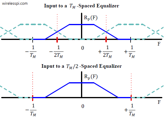
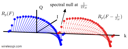
- Symbol-spaced equalizers are also commonly denoted as $T_M$-spaced equalizers. A tap spacing equal to the symbol time $T_M$ is optimum if the equalizer is preceded by an actual matched filter, i.e., a filter matched to the composite channel $h(nT_S)$ and not just the pulse shape. However, this is not often the case. The sample rate of $1/T_M$ can create a spectral null for an incorrect timing offset, a situation we encountered during a discussion on timing synchronization. Notice the red lines depicting the baseband region in the figure below for a $T_M$-spaced equalizer and an overlap from the neighbouring aliases.
- In many situations, the channel response is unknown at the Rx, so the Rx filter is matched to the known pulse shape and a symbol rate sampling is not enough. Due to the adverse effects of wrong timing, it has been shown that a fractionally-spaced equalizer delivers better performance than a symbol-spaced equalizer at the cost of increased complexity. When employing a fractionally-spaced equalizer, it is a common practice to use $L=2$ samples/symbol and denote it as a $T_M/2$-spaced equalizer. Notice the red lines depicting the baseband region in the figure above in which there is no overlap from the neighbouring aliases.

While we make these deductions about SNR reduction in isolation, keep in mind that the powerful error correcting codes can recover a great deal of information buried in noise and hence a $T_M$-spaced equalizer suffices in many scenarios.
Preset versus Adaptive
You might have observed that a carrier phase, carrier frequency or a symbol timing error can be considered as a special case of a wireless channel. On an analogous note, we observe the following.
- A regular equalizer can be considered as general case of a phase, frequency or timing estimator in a feedforward scenario.
- An adaptive equalizer can be viewed as a general case of a phase, frequency or timing locked loop in a feedback setting. We can think of it as a loop with several arms all driven by a common mechanism, as shown in the figure below. A relevant analogy is an ordinary serpent compared to the Hydra, a multi-headed serpent in Greek mythology that is killed by Heracles as one of his $12$ labours.

Hence, an equalizer can compensate for a carrier phase offset, a small frequency offset or a symbol timing offset (in a fractionally-spaced scenario). Nevertheless, the update process will be seriously complicated. Furthermore, the dynamics of the carrier and timing loops are much faster than the equalizer since the loops behave like a single-armed equalizer. Moreover, decoupling the individual distortions and conquering them separately in an independent manner is beneficial in terms of system complexity and performance. Even with the asymmetric pulses arising from multipath, the timing locked loop plays a crucial role of tracking the clock frequency to prevent timing drift, as long as the TED output is stable enough to not jump around when the paths come and go due to the fading. The important point is that timing recovery still brings out the symbol rate periodicity which largely stays intact even after the channel convolution.
For these reasons, an equalizer usually follows the timing synchronization process so that both the equalizer and synchronizer are not competing with each other to steer the timing. Then, the equalizer can compensate for the remaining timing error. A carrier phase loop, on the other hand, can operate at the equalizer output.
Linear versus Non-Linear
An equalizer is the most demanding and resource intensive component of a conventional wireless Rx, see a Maximum Likelihood Sequence Estimation (MLSE) equalizer as an example. While the exact numbers depend on the specifications and subsequent implementation of the system, it can consume even 75% of the processing resources of a DSP machine! In high speed communication, it is impractical to remain busy processing a symbol within a certain window of time while many future symbols are arriving at the Rx. That will result in filling the buffer faster than emptying it. Therefore, it is imperative to explore simple solutions for mitigating the effect of the channel.
For this reason, an equalizer is commonly divided into two categories, linear and non-linear equalizers.
Linear equalizers
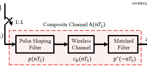
Linearity implies that the equalizers produce symbol estimates $y[m]$ based on simple linear operations on the matched filter output $z[m]$ (see the top figure for notations) and hence are inherently fast. The tradeoff is a higher bit error rate as well as an inability to effectively cope with harsh channels.
Non-linear equalizers
In this category, the equalizers generate the symbol outputs through more complicated mathematical operations than simple linear operations. On the up side, they perform significantly better in dealing with a frequency selective channel than linear equalizers in terms of the output bit error rate.
Time versus Frequency Domain
We have learned that equalization complexity is higher than any other signal processing task in a high rate wireless system. It turns out that beyond a certain rate, it is better to transform the signal into frequency domain through an FFT-iFFT pair and equalize the channel in frequency domain. With an ever growing demand for higher data rates, equalization in frequency domain has been the force behind most modern wireless standards.
Data-Aided/Decision-Directed versus Blind
Like synchronizers, many equalizers start their operation by processing a known training sequence embedded within the Rx signal. It is expected that at the end of training, the equalizer has reduced the channel impact to a level where it can switch to a decision-directed mode. Then, it can continue the process either until the end of the packet for burst transmissions or indefinitely for continuous transmissions.
On the other hand, blind equalizers work without any knowledge of the data or the channel and switch into a decision-directed mode only after crossing a certain threshold for convergence.
Finally, some equalizers require the knowledge of the channel impulse response at the Rx while many others do not. This requirement will become clear from the context of the algorithm.
All these categories are summarized in the figure below.

Simple and clear explanation, thank you.