Maximum Likelihood Sequence Estimation (MLSE Equalizer)

In the discussion on a wireless channel, we saw that an increased amount of Inter-Symbol Interference (ISI) occurs for high data-rate wireless systems that impacts the system performance to a significant extent.

• The performance of a linear equalizer suffers from spectral nulls.
• A Decision Feedback Equalizer (DFE) recovers much of the performance losses due to ISI but it is susceptible to error propagation.

In 1972, David Forney published a paper titled "Maximum-likelihood sequence estimation of digital sequences in the presence of intersymbol interference" in which he proposed the idea of sequence estimation. For this purpose, there was an implicit assumption that the input signal has been filtered through an exact matched filter as well as noise whitening filter for optimal performance. Without any knowledge of the channel, we just utilize a regular matched filter $p(-nT_S)$ in this setup. Furthermore, since measuring the performance is not our main goal, we ignore the noise whitening filter in this discussion.

System Model

---

As before, the modulation symbols are denoted by $a[m]$ while the channel response is represented as $h[m]$, where $m$ is the symbol index. A block diagram of such a structure is drawn in the figure below that shows a composite channel consisting of a pulse shaping filter, a baseband channel and a matched filter.

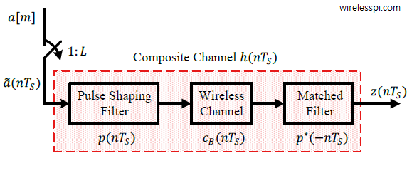
While the receiver input is denoted by $z(nT_S)$ where $1/T_S$ is the sample rate, the model for a symbol-spaced signal at 1 sample/symbol can be obtained by downsampling the above relation.
\begin{equation}\label{eqEqualizationTMchannelOut}
z[m] = a[m] * h[m]
\end{equation}

Basic Idea

---

Now although we do not have any knowledge of the Tx symbols $a[m]$ at the Rx, we do know that they come from a finite set of size $M$ depending on the modulation type. For example, $M$ is equal to $2$ in BPSK and $4$ in QPSK modulation. For a binary modulation scheme ($M=2$) and three data symbols ($N=3$) as an example, we get $M^{N}=2^3=8$ options as shown in the figure below.

Also, the channel impulse response can be known through any channel estimation strategy. Armed with this knowledge, we can convolve the channel impulse response estimate $\hat h[m]$ with all possible options for the symbol sequence $\tilde{a}[m]$ at the Rx. As a result, we get $M^{N}=2^3=8$ possible Rx sequences.

\begin{align*}
\tilde z_0[m] ~=~ \tilde a_0[m] *\hat h[m]\\
\tilde z_1[m] ~=~ \tilde a_1[m] *\hat h[m]\\
\tilde z_2[m] ~=~ \tilde a_2[m] *\hat h[m]\\
\tilde z_3[m] ~=~ \tilde a_3[m] *\hat h[m]\\
\\
\tilde z_4[m] ~=~ \tilde a_4[m] *\hat h[m]\\
\tilde z_5[m] ~=~ \tilde a_5[m] *\hat h[m]\\
\tilde z_6[m] ~=~ \tilde a_6[m] *\hat h[m]\\
\tilde z_7[m] ~=~ \tilde a_7[m] *\hat h[m]\\
\end{align*}

Let us call each such option $\tilde z_i[m]$ a candidate sequence. Then, a strategy is to use a slightly more general concept than correlation, i.e., we can find the error magnitudes between the Rx sequence $z[m]$ and the candidate sequences $\tilde z_i[m]$.
\begin{equation}\label{eqEqualizationMLSEerror}
e_i = \sum _m \big|z[m] – \tilde z_i[m]\big|^2
\end{equation}

The mostly likely Tx sequence is the one with the smallest such error. Note that the cross term $z^*[m] \tilde z_i[m]$ represents the correlation when we open the magnitude squared expression. The term $|z[m]|^2$ is common to all the error terms and hence not needed. However, the term $|\tilde z_i[m]|^2$ comes in due to different energies involved and subsequently required in addition to the correlation expression.

It turns out that this strategy is optimal in the sense of maximizing the likelihood of detected symbols in the presence of AWGN (as such a correlation process should do) and hence known as Maximum Likelihood Sequence Estimation (MLSE).

The Viterbi Algorithm

---

The significant disadvantage of this approach is its computational complexity. For a sequence length $N$ and modulation size $M$, there are $M^{N}$ possible sequences which is usually a very very large number. Even for a binary modulation with $M=2$ and a data length of just $10$ symbols, this is equal to $2^{N}$ $=$ $1024$ candidate sequences to compare!

To overcome this problem, the most widely known algorithm in digital communications, the Viterbi algorithm, can be employed. Viterbi algorithm breaks this process down in stages and works by only retaining the most likely candidates at each step. We discuss the Viterbi algorithm with the help of a simple setup of a binary modulation and a $2$ tap channel. From Eq (\ref{eqEqualizationTMchannelOut}), we can write
\begin{equation*}
z[m] = a[m] h[0] + a[m-1]h[1]
\end{equation*}

Let one term from the error sum in Eq (\ref{eqEqualizationMLSEerror}) be the metric
\begin{equation*}
M\{a[m],a[m-1]\} = \Big|z[m] – a[m] h[0] – a[m-1]h[1]\Big|^2
\end{equation*}

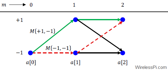
Now consider a diagram known as a trellis in the figure below.

• At time $m=0$, let $a[0]=-1$ be a single known training symbol and we need to detect the remaining symbols for $m>0$.
• At time $m=1$, there are two possible values for the metric $M\{a[1],a[0]\}$ because $a[1]$ can attain a value of either $+1$ or $-1$. These two metrics correspond to two different branches drawn in the above figure between $m=0$ and $m=1$. We say that the two branches end in two `states’ that depend on the possible values for $a[1]$.
• At $m=2$, there are now four possible branches, two from each state, corresponding to the possible values for the symbol pair $(a[1],a[2])$. Observe from the figure that two branches end at the state corresponding to $a[2]=-1$ while two end at the sate corresponding to $a[2]=+1$. The Viterbi algorithm dictates that at each state, only the sequence with minimum error is kept and the other is pruned. This minimum error is determined by the candidate \bbf{path metrics} which are an accumulation of $M\{a[m],a[m-1]\}$. And the process continues.

As an example, at state corresponding to $a[2]=+1$, there are only two possibilities for $a[1]$ since $a[2]$ is already determined.
\begin{equation*}
a[2]=+1\qquad \rightarrow \qquad a[1] = +1 ~~\text{or} ~~ a[1] = -1
\end{equation*}

Since $a[0]=-1$, the corresponding candidate metrics are as follows.
\begin{align*}
a[2],a[1] \quad~ & ~~~~\qquad a[1],a[0] \\
\\
\hline & \hline \\
M\{+1,+1\} \quad &+ \quad M\{+1,-1\} \\
M\{+1,-1\} \quad &+ \quad M\{-1,-1\}
\end{align*}

where the former is shown as a solid green line while the latter as a dashed red line from $a[0]$ to $a[2]$ in the above figure. The largest such metric determines which path is kept and its metric accumulated while the other is discarded. This results in each stage possessing a path history that determines the sequence for all the previous symbols. In the end, only the most likely sequence survives.

The benefit of the Viterbi algorithm over brute force sequence estimation is that we do not need to process all possible candidate sequences from the start to finish since the candidates are regularly discarded at each step. For a binary modulation scheme, length $L+1$ channel and data sequence length $N$, it reduces the brute force estimation of $2^{N}$ comparisons to $N$ stages of $2^{L}$ comparisons through discarding the trellis paths (keep in mind that $L+1$ is much smaller than $N$). Nonetheless, it is also prohibitive to implement in most wireless channels for realistic existing packet lengths, channel lengths and modulation sizes.

We feel a little annoyance when we forget an idea or something we are about to say. When that happens, starting with the last thought I remember, I list the next possible thoughts and compare how likely each of them can be. Keeping the one with highest likelihood, I repeat this process and often traverse the original route to capture what had escaped my mind. This could become Viterbi algorithm if I had some mechanism to incorporate an accumulation of path metrics.

A common use of maximum likelihood sequence estimation is during the design stage of the Rx, against which the potential performance of any equalization technique is benchmarked.