Imagine an alien race looking at our planet from outside the solar system through a lens of time. They will notice one unmistakable direction. Our pursuit of MORE in everything. This tendency might be ingrained in the fundamental idea of life itself. To live is to grow.
While our dreams for faster transportation face mechanical roadblocks from the laws of physics, technologies for faster communication are only bound by the laws of electromagnetics. Ever since we linked digital electronics to information exchange from one point to another without any physical medium, on-demand reception and transmission of data at any place and any time are exploding in an exponential manner. The obstacles encountered on this growth curve have consistently been overcome through invention of new technologies, some of which form the backbone of the physical layer (PHY) of 5G cellular systems. Massive MIMO is one of them.
Background
Increasing the number of antennas on wireless devices for enhancing performance is not a new discovery. However, in the initial years of wireless revolution, it was easier to grow the network capacity through a higher cell density (more number of base stations) and a wider spectrum. Nevertheless, the demand for more wireless traffic in the subsequent years required more innovation in the system design itself, which is where multiple antennas enter the picture.
In an older article, we saw several ways in which multiple antennas can improve the performance of a wireless communication system. As a consequence, base stations in cellular networks are now equipped with antenna arrays thus creating an opportunity to simultaneously communicate with several users at the same time and frequency. This is known as a Multi-User MIMO (MU-MIMO) system.
Now it is also possible to have multiple antennas at the user terminals but it is desirable to keep them simple and efficient with only a few antennas (at most). This number depends on the frequency of operation too. In sub-6 GHz band, the wavelengths are large (on the order of several centimeters) and since antenna spacing is a function of the wavelength, there is a limit to which antennas can be packed in the small form factor of mobile devices. On the other hand, mmWave frequencies allow a relatively large number of antennas in the handsets as well.
On the other hand, the trend is to assign the major cost and complexity of both the hardware and signal processing to the base station with a massive antenna array. This is where MU-MIMO forms the basis for massive MIMO. Since the users are geographically separated, their flat fading channel gains or spatial signatures are different from each other. This can be exploited by the base station array to generate multiple streams directed towards the users in an individual manner, sometimes called Space Division Multiple Access (SDMA).
A multi-user MIMO system offers some advantages as well as some drawbacks as follows.
- Customer terminals with a few antennas are simple in terms of hardware complexity, battery life and cost. Moreover, a rich scattering channel supports multiple data streams from multiple antennas because the user terminals are geographically scattered around the cell.
On the other hand, the drawbacks are as follows.
- While the hardware complexity is avoided in simple terminals, signal processing complexity at the user end still remains. For instance, users need to implement computationally intense detection algorithms (e.g., successive interference cancellation). This puts a drain on power budget of the user equipment. In a Frequency Division Duplex (FDD) system, not only the base station but each user must also know the channel coefficients for decoding the data in the downlink transmission, an approach that requires extra overheads.
This leads us towards the massive MIMO concept.
Massive MIMO
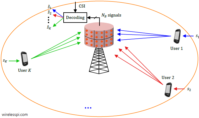
Consider a cellular network in which a single base station equipped with $N_B$ antennas serves $K$ user terminals, each of which has at most a few antennas. A block diagram for downlink of such massive MIMO systems is shown in the figure below.

While a massive MIMO system shares many of the features with a multi-user MIMO system described before, there are a few distinguishing features as follows.
- Observe from the block diagrams that the number of base station antennas $N_B$ is much larger than the number of users $K$.
- On both uplink and downlink, every transmission utilizes all the available time and frequency resources.
- The asymmetry between $N_B$ and $K$ facilitates simple linear processing at both the downlink and the uplink, as opposed to complex signal processing algorithms required for data detection in multi-user MIMO systems. More on this soon.
- In a Time Division Duplex (TDD) system, the user terminals do not have to learn about the channel coefficients to decode their data streams. It is sufficient for the Channel State Information (CSI) to be available at the base station only. This is not true for a more desirable FDD mode of operation.
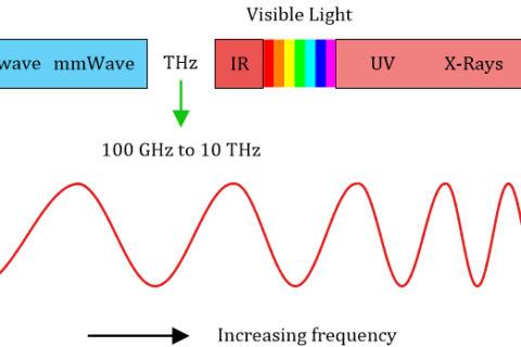
- While the idea was originally conceived for sub-6 GHz range, massive MIMO is even more more important for mmWave systems where the frequency span is from 30 to 300 GHz. This is because a smaller wavelength enables a large number of antennas to be integrated with the radio that provide significant Tx/Rx gains to help close the link.
Let us now explore how such an asymmetric arrangement facilitates simple algorithms for signal detection.
Spatial Matched Filtering (Maximum Ratio)
One of the most attractive features of massive MIMO is that simple linear algorithms can be employed for detecting the transmitted signal that translates into a significant reduction of computational load at the base station. This is in line with our tendency to spend more upfront (but only once) instead of incurring repeated costs of computationally complex signal processing algorithms. Let us see how this can be accomplished.
Setup
Consider the block diagram for uplink of a massive MIMO system as drawn below.
It is evident that the cumulative signal at each base station antenna $j$ is a summation of signals arriving from each user terminal $i$. While the expression below looks complicated, observe from the figure that the signal at each antenna is simply a sum of individual modulation symbols $s_1$, $s_2$, $\cdots$, $s_K$ scaled by channel coefficients.
$$\begin{equation}
\begin{aligned}
r_j = h_{(1\rightarrow j)}\cdot s_1 + h_{(2\rightarrow j)}\cdot s_2 + \cdots + h_{(K\rightarrow j)}\cdot s_{K} +~&~ \text{noise}, \qquad \\
& \qquad j = 1, 2, \cdots,N_B
\end{aligned}
\end{equation}\label{equation-massive-mimo-detection}$$
Here, the flat fading channel gain between $i$-th user terminal ($i=1,2\cdots,K$) and $j$-th base station antenna ($j=1,2,\cdots,N_B$) is denoted by $h_{(i\rightarrow j)}$. A word of caution: Power control is ignored here for simplicity. The reader should keep in mind that power control is important in cellular systems to prevent signals from users with strong channels drowning the signals coming from weak users. However, power control coefficients depend on large-scaling fading that renders them independent of both frequency and fast update rates.
Eq (\ref{equation-massive-mimo-detection}) tells us that the original signal received at the base station is not coming from terminal 1 alone! Instead, all user terminals transmit simultaneously on the uplink and hence the cumulative signal $r_j$ at each antenna $j$ is a superposition of signals from $K$ terminals. As a result, interference from $K-1$ users is added to the desired signal. The main task of the detection algorithms here is to free each modulation symbol $s_i$ sent by a user terminal $i$ from the interference of the other modulation symbols sent by rest of the mobile users. We explore these ideas next.
Detection Process
The simplest of linear processing techniques is spatial matched filtering, also known as conjugate beamforming, which are other terms used for Maximum Ratio Combining (MRC) or transmission. To understand the idea, let us consider the detection process through the perspective of mobile user 1.
Due to the large number of antennas, a figure is drawn to avoid any confusion between the input to the detection algorithm and the desired output. We have the received signals $r_j$ at $N_B$ antennas as the input and an estimate of its modulation symbol $\hat s_1$ as the desired output for user 1.

Assume that perfect channel estimates $h_{(i\rightarrow j)}$ are available at the base station. Also, the decoding vector for a specific terminal, say user 1, consists of weights $w_{1,j}$ that are complex conjugates of $h_{(1\rightarrow j)}$ (the channel gain from the single antenna of terminal 1 to the base station antenna $j$).
\[
w_{1,j} = h_{(1\rightarrow j)}^*, \qquad \qquad j = 1, 2, \cdots, N_B
\]
What happens when we apply these weights $w_{1,j}$ to the available inputs $r_1$, $r_2$, $\cdots$, $r_{N_B}$? Let us explore this scenario for the signal at the first base station antenna given by $r_1$ as illustrated in the figure below which only shows the signal $r_1$ received at the first base station antenna. Similar receptions for other antennas are not plotted to keep the figure clear.

From Eq (\ref{equation-massive-mimo-detection}),
\[
r_1 = h_{(1\rightarrow 1)}\cdot s_1 + h_{(2\rightarrow 1)}\cdot s_2 + \cdots + h_{(K\rightarrow 1)}\cdot s_{K} + \text{noise}
\]
After multiplying this with $w_{1,1}=h_{(1\rightarrow 1)}^*$, we get
$$\begin{equation}
\begin{aligned}
h_{(1\rightarrow 1)}^*\cdot r_1 &= h_{(1\rightarrow 1)}^*\cdot h_{(1\rightarrow 1)}\cdot s_1 + h_{(1\rightarrow 1)}^*\cdot h_{(2\rightarrow 1)}\cdot s_2 + \cdots + h_{(1\rightarrow 1)}^*\cdot h_{(K\rightarrow 1)}\cdot s_{K} + \text{noise} \\
&= \underbrace{|h_{(1\rightarrow 1)}|^2\cdot s_1}_{\text{Desired Signal}} + \underbrace{\sum \nolimits_{i=2}^{K} h_{(1\rightarrow 1)}^*\cdot h_{(i\rightarrow 1)}\cdot s_i}_{\text{Interference}} + \text{noise}
\end{aligned}
\end{equation}\label{equation-mami-r1}$$
Notice that the above summation in the interference part is with respect to user terminals $i$, not base station antennas $j$. Also keep in mind that $r_1$ is simply the first antenna at the base station which has no relation to user 1. Instead, we eventually take the outputs from all $N_B$ antennas. For instance, a similar equation at antenna $j=2$ can be written as
$$\begin{equation}
\begin{aligned}
h_{(1\rightarrow 2)}^*\cdot r_2 &= h_{(1\rightarrow 2)}^*\cdot h_{(1\rightarrow 2)}\cdot s_1 + h_{(1\rightarrow 2)}^*\cdot h_{(2\rightarrow 2)}\cdot s_2 + \cdots + h_{(1\rightarrow 2)}^*\cdot h_{(K\rightarrow 2)}\cdot s_{K} + \text{noise} \\
&= \underbrace{|h_{(1\rightarrow 2)}|^2\cdot s_1}_{\text{Desired Signal}} + \underbrace{\sum \nolimits_{i=2}^{K} h_{(1\rightarrow 2)}^*\cdot h_{(i\rightarrow 2)}\cdot s_i}_{\text{Interference}} + \text{noise}
\end{aligned}
\end{equation}\label{equation-mami-r2}$$
What happens when we average the weighted outputs from all $N_B$ antennas?
- Imagine a vertical summation on the left side of Eq (\ref{equation-mami-r1}) and Eq (\ref{equation-mami-r2}). The average operation on these terms yields
\begin{align}
\text{L.H.S.} =& \frac{1}{N_B}\Bigg\{h_{(1\rightarrow 1)}^*\cdot r_1 + h_{(1\rightarrow 2)}^*\cdot r_2 + \cdots + h_{(1\rightarrow N_B)}^*\cdot r_{N_B}\Bigg\}\nonumber \\=& \frac{1}{N_B}\sum \nolimits _{j=1}^{N_B} h_{(1\rightarrow j)}^*\cdot r_j \label{equation-lhs}
\end{align} - Imagine a vertical summation on the right side of Eq (\ref{equation-mami-r1}) and Eq (\ref{equation-mami-r2}). The average operation then gives the desired signal and interference as
\begin{equation}\label{equation-rhs}
\text{R.H.S.} = \frac{1}{N_B}\sum\nolimits _{j=1}^{N_B} \Bigg\{ \underbrace{|h_{(1\rightarrow j)}|^2 s_1}_{\text{Desired Signal}}+ \underbrace{\sum\nolimits _{i=2}^{K}h_{(1\rightarrow j)}^*\cdot h_{(i\rightarrow j)} s_i}_{\text{Interference}} \Bigg\}
\end{equation}These operations are illustrated in the figure below. While the figure looks complicated, you can follow the expressions above and focus on user 1 only to understand this block diagram.

Next, the impact of this combination on the desired signal and the interference part can now be investigated as follows.
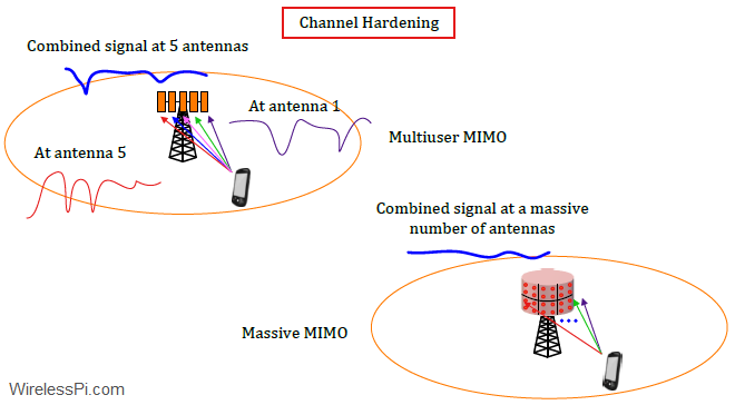
Channel Hardening
From Eq (\ref{equation-rhs}), the sum of the weighted outputs from all antennas yields the desired signal part in the first term as
\begin{align}
\text{Desired Signal} &= \frac{1}{N_B}\sum \nolimits_{j=1}^{N_B} |h_{(1\rightarrow j)}|^2 \cdot s_1 \label{equation-effective-channel} \\ &\approx s_1 \qquad \text{for large }N_B \label{equation-desired-signal}
\end{align}
Both of the above two steps require some explanation.
- Eq (\ref{equation-effective-channel}): With proper weighting, notice that the effective channel from terminal 1 at the output of the decoder becomes $\sum \nolimits_{j=1}^{N_B} |h_{(1\rightarrow j)}|^2$. The above expression is the Maximum Ratio Combining (MRC) or beamforming towards all $N_B$ antennas from the intended user 1 that aligns the phases and grades the magnitudes for each channel. This gain and phase matching according to the channel gains from user 1 maximizes the signal power accumulated from that particular transmission. And that is why it is also known as spatial matched filtering in the context of massive MIMO detection.
- Eq (\ref{equation-desired-signal}): When the base station has a large number of antennas $N_B$, we get
\begin{equation}\label{equation-channel-hardening}
\frac{1}{N_B}\sum \nolimits_{j=1}^{N_B} |h_{(1\rightarrow j)}|^2 \quad\rightarrow\quad \text{Avg}~\left\{|h_{(1\rightarrow j)}|^2\right\}\quad\rightarrow\quad 1
\end{equation}where we have assumed normalized channel gains. By virtue of the law of large numbers, summing a large number of channel gains on the left side generates the arithmetic mean or average value over those gains that is a constant number. This phenomenon is known as channel hardening.
Massive MIMO benefits from channel hardening because it simplifies the signal processing and resource allocation at the base station. Looking back at Eq (\ref{equation-channel-hardening}), observe that there is very little fluctuation in the cumulative channel from each terminal at the base station as this expression mostly converges towards a constant value (while this is shown as $1$ here, the actual value depends on large-scale fading). The channel hardening idea is illustrated in the figure below. The signal received at each antenna undergoes small-scale fading and fluctuates rapidly over a short time interval. This is due to the multipath nature of the channel described here. However, the combined signal starts to smooth out when inputs at multiple antennas is taken into account. In MU-MIMO case at the top of this figure, the channel variations, though reduced, are still visible. On the other hand, the massive MIMO setup at the bottom of this figure plots the combined signal from a large number of antennas and shows no signs of rapid fluctuations.

The benefits achieved through channel hardening in a massive MIMO system are as follows.
Fading Vanishes: A constant output or the absence of channel fluctuations in time implies that the small-scale fading practically disappears! In other words, such an ideal system provides average SNR all the time as instantaneous SNR. If the probability of failure is given by $p$, then the probability of all paths simultaneously going down is given by
\[
P(\text{success}) = 1 – P(\text{failure}) = 1 – p^L \quad \rightarrow \quad 1
\]
With a large $L$, the probability of success goes to 1 since $p$ is between 0 and 1.
As a consequence, a Rayleigh fading channel is transformed into more like an AWGN one and several tens of dB more SNR theoretically required to cover the BER performance gap between AWGN and fading channels is reclaimed. In addition, this phenomenon enables a significant reduction of latency on the air interface because fading is the major bottleneck in building low-latency wireless networks.
Frequency Independence: Since the effective channel reduces to a constant value, there is no more frequency dependence for the channel gains. To understand this idea, recall that channel delay spread is determined by the last and first most significant paths. Considering the downlink case, the precoding weights compensate for the time delays for narrowband signals (an idea we covered in beamforming). Consequently, the delay spread is compensated for by the base station through precoding before the transmission and the effective channel impulse response reduces to a single tap. In frequency domain, a small delay spared gives rise to a large coherence bandwidth and the flat channel becomes deterministic with respect to small variations. A similar effect is observed through combining after the reception on the uplink.
Uniformly Good Service: In 4G (and previous generations of cellular networks), resource allocation was not a straightforward task since different users face different channel conditions as a function of frequency and a suitable modulation and coding scheme is selected accordingly (e.g., for each subcarrier in OFDM case). This is shown in the figure below where each subcarrier in an OFDM system encounters a different level of channel fade.

A huge implication of the frequency independence in massive MIMO is the simplification of the multiple access strategy. It becomes possible for the base station to provide uniformly good service to all users in a simultaneous manner through large-scale fading power control. A uniformly good service simplifies not only resource allocation but also the signal processing complexity.
Channel Code: The role of a channel code in digital communication systems is to protect the data against noise and interference at the Rx with the purpose of avoiding retransmissions of the same information. Different strategies are applied for designing a channel code for a wireless channel as compared to a simple AWGN channel. One consequence of the above channel transformation is that standard modulation and coding schemes designed for AWGN also work well with the fading channels.
Channel Estimation From a theoretical viewpoint, due to channel hardening, channel estimation at the terminals is mostly not required for signal detection because the receiver only needs the statistical knowledge of the channel gains (instead of their instantaneous values) from large-scale fading. This eliminates the need for downlink pilots transmission and saves power and training duration otherwise needed for channel estimation. This is an oversimplification that does not hold in many circumstances. Also keep in mind that massive MIMO systems suffer from pilot contamination problem.
Favorable Propagation
From Eq (\ref{equation-rhs}), the interference part that comes from the sum of weighted outputs from all antennas yields
\begin{align}
\text{Interference} &= \sum \nolimits_{i=2}^{K} \underbrace{\frac{1}{N_B}\sum \nolimits_{j=1}^{N_B} h_{(1\rightarrow j)}^*\cdot h_{(i\rightarrow j)}}_{\rightarrow ~0\text{ for large }N_B}\cdot s_i \label{equation-favorable-propagation-2} \\ &\rightarrow 0
\end{align}
The last expression $\frac{1}{N_B}\sum \nolimits_{j=1}^{N_B} h_{(1\rightarrow j)}^*\cdot h_{(i\rightarrow j)}$ goes to zero because
- each factor $h_{(i\rightarrow j)}$ including $h_{(1\rightarrow j)}$ is a complex random variable with a zero mean, and
- averaging the product of a large number of such random variables makes the numerator grow slower ($\sqrt{N_B}$ for Gaussian distribution) than the denominator $N_B$ and hence the expression converges towards zero.
This is known as asymptotic favorable propagation exhibited by real wireless channels in which such a sum of products goes to zero when normalized with the number of base station antennas $N_B$. That then holds true even when the fading channel coefficients assume any non-Gaussian distribution as well. In academic works, however, using strictly favorable propagation without any normalization with $N_B$ is more common due to its analytical tractability. In any case, favorable propagation is how massive MIMO achieves user separation in a cell through identifying their different spatial signatures
Eq (\ref{equation-channel-hardening}) and Eq (\ref{equation-favorable-propagation-2}) can now be combined into a single expression for a user $i’$ as
\frac{1}{N_B}\sum \nolimits_{j=1}^{N_B} h_{i’\rightarrow j}^*\cdot h_{(i\rightarrow j)} \quad \rightarrow \quad \left\{ \begin{array}{l}
1, \quad~~~ i’=i \\
0, \quad ~~~\text{otherwise} \\
\end{array} \right.
\end{equation}
where we have used the fact that $h_{(i\rightarrow j)}^*\cdot h_{(i\rightarrow j)}$ $=$ $|h_{(i\rightarrow j)}|^2$ which was normalized to $1$ as before. In words, favorable propagation means that user transmissions in the presence of decoding and precoding vectors virtually act as if each terminal is communicating alone with the base station, an idea known as orthogonality. This helps separating the users in spatial domain despite the fact that they share all the available time and frequency resources.
Finally, combining the left and right hand expressions in Eq (\ref{equation-lhs}) and Eq (\ref{equation-rhs}), the estimate at the base station with respect to user 1 data generates the output
\hat s_1 = \frac{1}{N_B}\sum \nolimits _{j=1}^{N_B} h_{(1\rightarrow j)}^*\cdot r_j
\]
which is a simple linear expression! This is largely due to channel hardening and favorable propagation phenomena. This is why simple linear processing on signals can (ideally) achieve nearly optimal performance in a massive MIMO system.
On the uplink, a simple matched filter or maximum ratio combining (in the form of proper decoding vectors as described above) can overcome noise and interference for signal detection. Here, the signal model becomes multi-dimensional as
\[
\mathbf{r} = \mathbf{H}\cdot \mathbf{s} + \mathbf{\text{noise}}
\]
where $\mathbf{r}$ is a vector of received samples $r_j$, $\mathbf{H}$ is a matrix whose entries $h_{(i\rightarrow j)}$ are channel gains from user $i$ to antenna $j$ and $\mathbf{s}$ is the vector of modulation symbols $s_1$, $s_2$, $\cdots$, $s_K$. Just like we multiplied the samples $r_j$ with $h_{(1\rightarrow j)}$ for user 1, the decoding vectors for all $K$ users can be combined into an $N_B$ $\times$ $K$ matrix $\mathbf{H}$. The matched filter detector can thus be written as
\begin{equation}\label{equation-mf-detector}
\mathbf{\hat s} = \mathbf{H^*\:r}
\end{equation}
where $\mathbf{H^*}$ here represents both a transpose and a conjugate operation on channel matrix $\mathbf{H}$ (technically, both transpose and conjugate are incorporated as $\mathbf{H^H}$ known as the Hermitian of a matrix but I preferred to avoid including another mathematical operation).
As far as the downlink is concerned, a similar precoding vector for each user enables the base station to beamform multiple data streams to all user terminals without causing significant mutual interference among them. The mobile terminal does not have to carry out the decoding part as the summation in the term $\hat s_1$ is automatically done by nature at the Rx antenna. This is very important in a multiuser system since the individual users do not have any information about channel gains of others and hence cannot suppress their interference.
In summary, with the help of channel hardening and favorable propagation, massive MIMO effectively creates dedicated virtual pipes between a base station and its terminals where the frequency independent channel can be simply determined through large scale fading and power control. Another linear detection technique, known as Zero-Forcing (ZF), is explained here.
How to get this article in pdf format