In the discussion on diversity, we described in detail the idea of space diversity through an example of Selection Combining (SC). Maximum Ratio Combining (MRC) is another space diversity scheme that embodies the concept behind generalized beamforming — the main technology in 5G cellular systems. Let us find out how.
Setup
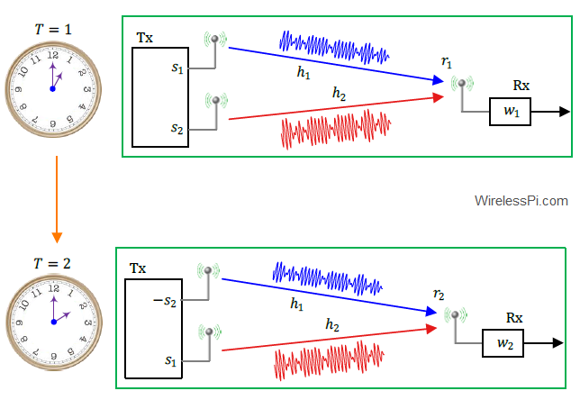
Consider a wireless link with 2 Tx antenna and 2 (or more) Rx antennas as shown in the figure below. At each symbol time, a data symbol $s$ is transmitted which belongs to a Quadrature Amplitude Modulation (QAM) scheme. To focus on the events happening within one symbol time only, we have dropped the time index $m$ from the modulation symbol $s[m]$ here.

- In this setup, $r_1$ is the signal received by the first antenna while $r_2$ is the signal received by the second antenna.
- $h_1$ is the flat fading channel gain between the Tx antenna and the first receive antenna.
- $h_2$ is the flat fading channel gain between the Tx antenna and the second receive antenna.
Consequently, the expressions for the signals at the Rx is given by
\begin{equation}
\begin{aligned}\label{equation-simo}
r_1 &= h_1\cdot s + \text{noise} \\
r_2 &= h_2\cdot s + \text{noise}
\end{aligned}
\end{equation}
Here, the channel gains $h_1$ and $h_2$ are usually modeled as complex Gaussian random variables.
Why a Simple Summation Will Not Work
In selection combining, we simply scan the power arriving at each antenna and choose the one with the highest SNR. However, selecting the antenna with the best SNR implies that energy at the other antennas is neglected. Instead, the design goal can be modified to maximize the SNR by scavenging the energy from all Rx antenna streams. As we now see, picking additional spatial samples from the air is not enough. We must know how to efficiently utilize them.
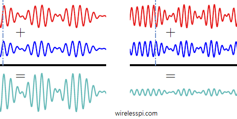
The first idea then is to sum the signal from all these antennas. Recall that the channel gains $h_1$ and $h_2$ are complex Gaussian random variables here. This in turn implies that their magnitudes are Rayleigh distributed and phases are uniformly distributed between $0$ and $2\pi$. Therefore, adding several complex numbers with random phases tends to average out the summation!
Computing the Weights $w_i$
In this spirit, a Maximum Ratio Combining (MRC) receiver is also drawn in the figure above that forms the decision through a linear combination of $r_1$ and $r_2$ after weighting them with complex scalars $w_1$ and $w_2$, respectively. The output signal $z$ is given by
$$
\begin{equation}
\begin{aligned}
z &= w_1\cdot r_1 + w_2 \cdot r_2 + \text{noise} \\
&= w_1\cdot h_1\cdot s + w_2 \cdot h_2 \cdot s + \text{noise}\\
&= s\cdot \left\{ w_1\cdot h_1 + w_2 \cdot h_2\right\} + \text{noise}
\end{aligned}
\end{equation}\label{equation-mrc-combiner-1}
$$
The general expression for $N_R$ antennas can be written as
\begin{equation}\label{equation-general-z-w}
z = s\sum _{i=1}^{N_R} w_i\cdot h_j + \text{noise}
\end{equation}
Here, the effect of scaling by $w_j$ on the noise samples is ignored for simplicity. Also, while the parameters $w_j$ in classical beamforming were selected according to the signal direction of arrival or departure, a different criterion is chosen in virtual beamforming due to the absence of a single such direction owing to multipath nature of the wireless channel.
Each channel gain $h_j$ is a complex number with magnitude $|h_j|$ and phase $\measuredangle h_j$. Magnitudes and phases of $w_j$ can be represented in a similar manner. Then, we can write their complex product (in which magnitudes are multiplied while phases are added) below. In complex notation, this is written as
\[
w_j\cdot h_j= |w_j|\cdot|h_j|\cdot e^{j\left(\measuredangle w_j+\measuredangle h_j\right)}
\]
In terms of real signals,
$$ \begin{equation}
\begin{aligned}
|w_j\cdot h_j| &= |w_j|\cdot |h_j| \\
\measuredangle \left(w_j\cdot h_j\right) &= \measuredangle w_j + \measuredangle h_j
\end{aligned}
\end{equation}\label{equation-w-h-mrc}
$$
To see how optimal $w_j$ are chosen, assume that the channel gains $h_j$ are known at the Rx. In practice, this is usually accomplished through a channel estimation procedure by inserting a training sequence or periodic pilot symbols known at the Rx in the information stream. Then, we can proceed as follows.
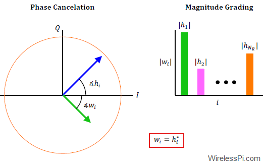
Canceling the Phase
If the weight $w_j$ has an opposite phase as compared to that of $h_j$, we have $\measuredangle w_j=-\measuredangle h_j$ and the complex multiplication will cancel out the phases, see Eq (\ref{equation-w-h-mrc}). On the other hand, noise samples simply add without any phase alignment. With this substitution, the combiner output from Eq (\ref{equation-mrc-combiner-1}) becomes
\begin{equation}\label{equation-phase-cancelation}
z = s\sum_{j=1}^{N_R} |w_j|\cdot|h_j| + \text{noise}
\end{equation}
where the effect of scaling by $w_j$ on the noise samples is ignored here. This phase cancellation is shown on the left of the figure below. All channel gains are said to be aligned at the Rx in the same direction. Since we have not yet modified the magnitude of $w_j$, all $w_j$ have unit magnitude here. This scheme is known as Equal Gain Combining (EGC).

Grading the Magnitude
It is obvious that the branches with better SNR provide a more reliable contribution towards making the modulation symbol decision. Therefore, the branches with higher SNRs should be given more weight as compared to the ones with less signal energy. I call this grading the magnitudes which is shown on the right of the figure above, similar to how the courses with higher credit hours contribute more towards a student’s GPA. In the algorithm, this can be accomplished by choosing $|w_j|$ the same as $|h_j|$ which is a measure of confidence for the channel gain at $i$-th Rx antenna.
\[
|w_j| = |h_j|
\]
When the magnitudes of $w_j$ are chosen according to the above expression, Eq (\ref{equation-phase-cancelation}) becomes
\begin{equation}\label{equation-mrc-magnitude}
z = s\sum_{j=1}^{N_R} |h_j|^2 + \text{noise}
\end{equation}
Notice how the energy from all the Rx branches is being summed in the above expression (without any detrimental effects that come from out-of-phase summations); this is generalized beamforming! As a consequence, this is the optimal approach for signal processing decisions and hence MRC performance is better than every other Rx diversity scheme.
This reminds me of the Brexit vote. Famous biologist Richard Dawkins said that the majority of the British public (including himself) should never have been asked to participate in that referendum. In his opinion, this decision was only up to those with necessary expertise in economics and history.
Taking an analogy from maximum ratio combining, estimation theory tells us that neither the public referendum nor Dawkins’ selective suggestion is an optimal approach. Instead, here is what should be done. Given the options in light of a common reference such as a country’s ideology or long term goals, everyone should vote in such decisions and every vote should be weighted (on a scale from 0 to 1) in proportion to the person’s expertise in the relevant matter.
In summary, since the conjugate of a complex number inverts its phase but leaves the magnitude unchanged, the optimal $w_j$ can be chosen as complex conjugates of $h_j$.
w_j = h^*_j
\end{equation}
To keep the expressions simple here, I have deliberately skipped the power normalization part where these $h^*_j$ are scaled by $1/\sqrt{\sum \nolimits_{j=1}^{N_R} |h_j|^2}$.
While complex conjugates are used for selecting the weights $w_j$, recall that a similar conjugate product was taken for physical beamforming scenario too! Nevertheless, there are two main differences here.
- In classical beamforming, the weights $w_i$ were chosen as conjugates in relation to the angle of arrival of the wave manifested by array response vector, thus enabling the beam to `look’ into particular directions. In generalized beamforming on the other hand, the weights $w_j$ are chosen as conjugates of the overall flat fading channel gains $h_j$. This introduces diversity in the system.
- Due to a planar wavefront assumption, the Rx signal at each antenna differed in phase only with no difference in magnitude. So the product $w_i\cdot a_i$ had a magnitude of $1$. On the other hand, all channel gains $h_j$ are not the same here and therefore a conjugate operation produces $w_j$ with varying magnitudes.
Having worked out the antenna weights $w_j$, let us apply the results to our initial setup of 1 Tx antenna and 2 Rx antennas. When these weights $w_j=h^*_i$ are applied to the Rx signal branches as in Eq (\ref{equation-mrc-combiner-1}), the resulting signal available for demodulation becomes
\begin{equation}\label{equation-mrc}
z = \left\{ h^*_1\cdot h_1 + h^*_2 \cdot h_2\right\}\cdot s + \text{noise} = \Big\{|h_1|^2+|h_2|^2 \Big\} \cdot s + \text{noise}
\end{equation}
since the product of a complex number with its conjugate cancels the phase and squares the magnitude (here, the noise term here is actually a superposition of two individual noise terms). For known normalized channel gains and a zero noise scenario, the symbol estimate $\hat s$ can be written from Eq (\ref{equation-mrc}) as
\begin{equation}\label{equation-mrc-s}
\hat s = \frac{z}{|h_1|^2+|h_2|^2}
\end{equation}

This estimate $\hat s$ maps exactly on one of the modulation symbols. When noise or other distortions are present, a 16-QAM example is also shown above where a decision is made in favour of the star nearest to the blue point $\hat s$. This is because the modulation symbol with the minimum distance from $z$ is the most likely candidate for a Gaussian noise distribution (because there is a squared Euclidean distance term in the exponential power of Gaussian probability density function).
Noncoherent Demodulation
In coherent demodulation, the Rx knows or estimates the channel gain or carrier phase. Noncoherent demodulation implies that the Rx has to detect the symbols without any knowledge of channel gain or carrier phase. An example for this scheme is Differential Phase Shift Keying (DPSK).
It seems that maximum ratio combining is only effective for coherent demodulation where the channel response is known. However, we see in the below example that MRC is also applicable to noncoherent receivers in some cases.
Consider an OFDM receiver with 8-DPSK modulated symbols riding on the subcarriers. The mathematical expression of the differential symbol is
\[
s_{j,n} = x_{j,n}\cdot x^*_{j,n-1}
\]
where $n$ is the time index and $j$ is the subcarrier index. Given that $h_{i,j,n}$ is the flat fading channel gain at time $n$, subcarrier $j$ and antenna $i$, we have
\[
z_{i,j,n} = h_{i,j,n}x_{j,n} + \text{noise}
\]
In vector form, for $N$ antennas, we have
\[
\begin{aligned}
\bar{z}_{j,n} &= [z_{1,j,n} z_{2,j,n} \cdots z_{N,j,n}] \\
\bar{h}_{j,n} &= [h_{1,j,n} h_{2,j,n} \cdots h_{N,j,n}]
\end{aligned}
\]
The optimal combiner is given by $w^T_{j,n}z_{j,n}$. Clearly, $||\bar{z}_{j,n} – \bar{h}_{j,n}x_{j,n}||^2$ is minimized for
\[
\hat x_{j,n} = (\bar{h}^*_{j,n}\bar{h}_{j,n})^{-1}\cdot \bar{h}^*_{j,n}\bar{z}_{j,n}
\]
With $\bar{w}_{j,n} = \bar{h}^*_{j,n}$, we get
\[
\bar{w}^T_{j,n}\bar{z}_{j,n} = \sum_{i=1}^{N}|h_{i,j,n}|^2x_{j,n}
\]
The question is how to detect the channel gains $\hat h_{i,j,n}$ which are not available in noncoherent demodulation.
But using differential detection, we already have $h_{i,j,n}$ $\approx$ $h_{i,j,n-1}$. Therefore, the maximum ratio combining can be applied by combining it with differential detection in one step as
\[
\hat s_{j,n} = \bar{z}^*_{j,n}\bar{z}_{j,n-1}
\]
This is because
\[
\bar{h}^*_{j,n}\cdot x^*_{j,n}\cdot \bar{h}_{j,n-1}x_{j,n-1} \approx \sum_{i=1}^{N}|h_{i,j,n}|^2s_{j,n} + \text{noise}
\]
This is very similar to MRC due to channel gain not effectively changing during the next symbol.
Hi – nice post. Not sure if I understood the “Phase cancelation” figure above. Are the phases of h and w cancelled out?
thanks
That’s right. As written above, “If the weight $w_j$ has an opposite phase as compared to that of $h_j$, we have $\measuredangle w_j=-\measuredangle h_j$ and the complex multiplication will cancel out the phases, see Eq (\ref{equation-w-h-mrc})”. This aligns both h and w along the real line with maximum gain.
This is an excellent idea. I am interested in MRC, but how can I exploit Genetic Algorithm as the MRC weighting parameter? Please. Thank you.
Hello! Thank you for the post. Does signal processing happen at the baseband or passband? And why we assume that the optimal weight is a conjugate of a channel, I understand that phases need to cancel out but why their magnitudes need to be equal?
My theory is that this way we ensure that signals with higher SNR get more weight and vice versa lower SNR corresponds to less weight.
1. Signal processing happens at baseband.
2. Your theory about SNR weightage is correct. In this way, the branch with higher SNR gives more contribution to the final estimate.