Channel estimation in single-carrier systems has been described in a previous article. In OFDM systems, each subcarrier acts as an independent channel as long as there is no Inter-Carrier Interference (ICI) left in the synchronized signal. The options of both a training sequence and individual pilots are available for channel estimation and the choice between the two depends on time variation rate of the channel as well as the computational complexity. Many systems acquire the channel through the preamble while employ the pilots for channel tracking. The discussion in this article is mostly based on Ref. [1].
For a simplified OFDM system model, the signal after the FFT at the receiver can be written as a product between the data symbols $a[k]$ and channel frequency response $H[k]$ at each subcarrier $k$.
\begin{equation*}
\begin{aligned}
Z[k] = a[k]\cdot H[k]~~& \\
&\hspace{-.5in}\text{for each }k = -N/2,\cdots,N/2-1
\end{aligned}
\end{equation*}
Based on this model, there are different estimation schemes as follows.
Training Based Estimation
In some systems, training OFDM symbols are periodically sent in the Rx signal so that the channel estimate can be updated at the same rate. In such a scenario, all subcarriers of an OFDM symbol are occupied by the training as shown in the figure below where OFDM symbols for $m=0$ and $m=4$ are the training symbols. After estimating the channel for the initial training sequence, it is common to assume a time-invariant channel (and hence valid estimates for subsequent OFDM data symbols) until the next training sequence arrives. Then, the channel estimate is updated and used again for subsequent OFDM symbols and this process is known as piecewise constant interpolation. For example, training based channel estimation is adopted in IEEE 802.11a/b/g and fixed WiMAX systems.

Since the symbols $a[k]$ are known in this context, we can write
\begin{equation}\label{eqOFDMLS}
\begin{aligned}
\hat H[k] = \frac{Z[k]}{a[k]}~~& \\
&\hspace{-.5in}\text{for each }k = -N/2,\cdots,N/2-1
\end{aligned}
\end{equation}
This is commonly known as Least Squares (LS) channel estimation which in case of OFDM subcarriers is also Maximum Likelihood (ML) solution. Depending on the channel characteristics and the system requirements, this can suffice alone or can be computed as a first estimate before refining it through a more advanced technique.
From the above figure, it is evident that frequency selectivity of the channel is not a problem due to its division into underlying flat fading subcarriers. Even if the channel is drastically different from one subcarrier to the next, it can satisfactorily be estimated by probing on all frequencies.
On the other hand, it is the time domain where the gaps are left and hence susceptible to time selectivity of the channel. Ideally, the training sequences need to be as far apart as possible to minimize the overhead and maximize the data rate. To find out the maximum required spacing between them, we refer to the sampling theorem. The period between two training sequences needs to be at least as frequent as the coherence time of the channel which is the inverse of the Doppler spread (normalized by subcarrier spacing).
Since the OFDM symbols between the training are used to deliver the data symbols, a decision-directed approach can also be employed to smooth the channel tracking between the training sequences.
Pilot Based Estimation
Another option is to insert regularly spaced pilots in some subcarriers that are kept occupied for each OFDM symbol. In this way, the pilots are multiplexed with the data and this arrangement is shown in the figure below. For example, the subcarriers $k=-2$ and $k=1$ are taken by the pilots here. Then, a similar equation as in training case can also be used for pilot-aided channel estimation for values of $k$ corresponding to the pilot symbols.

In this case, tracking rapid time variations of the channel is not a problem since the pilots are present for each OFDM symbol. On the other hand, there is a gap between them in the frequency domain and hence they are susceptible to frequency selectivity of the channel. For this purpose, the maximum gap between two pilots is governed by the coherence bandwidth.
As before, the data symbols between the pilots can be exploited in a decision-directed manner to improve on the channel estimates.
Optimal pilot locations
This is determined by the channel fading characteristics in time and frequency domains. Our objective is to insert a minimum number of pilots in the OFDM time-frequency grid. A larger number is a waste of power while a smaller number is a performance loss due to insufficient channel sampling. The tradeoffs involved are accuracy (the more, the better) and spectral efficiency (the lesser, the better). Once a certain number of pilots is determined, it has been reported that the minimum mean square error is obtained when the pilots are equispaced with maximum distance from each other.
Power and modulation
Many systems transmit more power at the pilot subcarriers than the data subcarriers. Also, a lower-order modulation scheme, such as BPSK, is well suited for pilot assignment since a higher data rate is not an objective and maximum power can be allocated to BPSK symbols instead of dividing it into $M$ PSK symbols for normalization, thus implying a longer range.
Interpolation
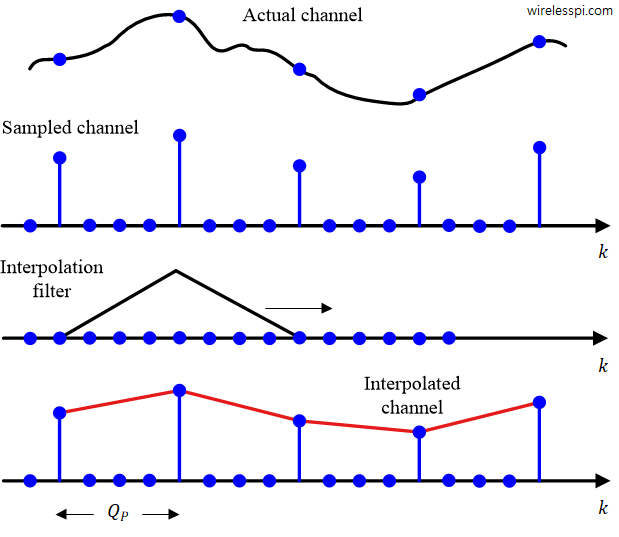
Interpolation between the pilot subcarriers can be carried out in both time and frequency domains. A piecewise constant interpolation technique that implies a constant channel between two training sequences can be employed. In the case of pilot subcarriers, linear interpolation offers better performance without adding much complexity to the block.
Assume that two pilot measurements are available at subcarriers $k=k_1$ and $k=k_2$ where
\begin{equation*}
k_2 – k_1 = Q_P
\end{equation*}
Then, we can find the channel estimate for any other $k$ by linear interpolation.
\begin{equation*}
\hat H(k) = \mu_k \hat H[k_1] + (1-\mu_k)\hat H[k_2], \qquad k_1 < k < k_2
\end{equation*}
where $\mu_k$ is given by
\begin{equation*}
\mu_k = \frac{k}{Q_P}
\end{equation*}
It can be viewed as a $2$ tap filter applied to the channel estimate sequence after upsampling the channel estimates at pilot locations by $Q_P$. This is shown in the figure below. Better interpolation techniques such as Wiener, Gaussian, cubic or spline are also frequently applied for this purpose. Finally, taking an iFFT/FFT pair also accomplishes pilot interpolation if the FFT size is divisible by the pilot spacing.

Another option is to arrange the pilots on adjacent subcarriers in adjacent OFDM symbols such that they cover the time-frequency grid in a diagonal fashion. This helps in sampling the channel at all times and all subcarriers in a periodic manner.
Transform Domain Techniques
There are scenarios in which the number of taps in the channel impulse response is much less than the Cyclic Prefix (CP) length. This extra information helps in refining an initial channel estimate (such as the Least Squares (LS) estimate) by concentrating on the channel taps within the delay spread and nullifying the effect of the noise outside the farthest channel tap.
Consider an OFDM system with the CP length $N_{CP}$ and the number of subcarriers $N$ operating in a channel with length $N_{Tap}+1$. Let $\hat H[k]$ for each subcarrier $k$ denote the Least Squares estimate for the corresponding channel gain. Next, we take the iFFT of $\hat H[k]$ and denote it by $\hat h[n]$ that represents an estimate of the channel impulse response $h[n]$. This sequence in time domain is given by
\begin{equation*}
\hat h[n] = h[n] + \text{noise}, \qquad n = 0,1,\cdots,N-1
\end{equation*}
Since the actual channel length is $N_{Tap}+1$, all the taps after $N_{Tap}$ consist of noise only. Here, we form a new channel estimate $\hat h_{FFT}[n]$ by removing all the taps from $\hat h[n]$ beyond $N_{Tap}$.
\begin{equation*}
\hat h_{FFT}[n] =
\begin{cases}
h[n] + \text{noise} & n = 0,1, \cdots, N_{Tap} \\
0 & n = N_{Tap}+1,\cdots,N-1
\end{cases}
\end{equation*}
Now when we perform an FFT of the above sequence to go back to the frequency domain, the resultant channel estimates are free of noise beyond $n=N_{Tap}$ and consequently yield better performance.
\begin{equation*}
\hat H_{FFT}[k] = \text{FFT} \Big\{\hat h_{FFT}[n]\Big\}
\end{equation*}
A block diagram for the implementation of such an approach is drawn in the figure below.

Although a similar concept can be applied to some other transforms, the FFT is particularly attractive due to its efficient implementation.
Decision-Directed Channel Estimation
Due to its widespread use in single-carrier systems, decision-directed channel estimation was one of the earliest methods explored for OFDM systems. It is particularly useful because after the initial estimates, the channel coefficients can be updated with the help of decisions from data symbols. The basic idea is to employ the channel estimates from the previous OFDM symbol to detect the data in the current OFDM symbol.
- Assume that the channel is slowly varying from one OFDM symbol to the next. Let $Z_m[k]$ be the $m^{th}$ Rx signal after the FFT and $\hat H_{m-1}[k]$ be the channel estimate for $(m-1)^{th}$ OFDM symbol. Then, it can be employed to detect the current data symbols as
- Next, the symbol candidate $\hat a[_m[k]$ can be used for estimating the channel $\hat H_m[k]$ at time $m$ as
\begin{equation*}
\hat H_m[k] = \frac{Z_m[k]}{\hat a_m[k]}
\end{equation*}As another option, the data symbol decision $\text{sign}$ $\{\hat a_m[k]\}$ can also be used for this purpose to reduce the effect of noise.
\begin{equation*}
\hat a_m[k] = \frac{Z_m[k]}{\hat H_{m-1}[k]}
\end{equation*}
\begin{equation*}
\hat H_m[k] = \frac{Z_m[k]}{\text{sign}\{\hat a_m[k]\}}
\end{equation*}
There are two main problems with this kind of decision-directed approach.
- Channel estimate expiry: For a quickly varying channel on a time scale of an OFDM symbol, the channel estimates at time $m-1$ are no longer valid at time $m$. Consequently, the detected symbols $\hat a_m[k]$ increasingly suffer from errors.
- Error propagation: Wrong data symbols fed back to estimate the current channel gives rise to error propagation which renders the system dysfunctional. This is a problem associated with all decision-directed techniques whether in the context of equalization or synchronization.
To resolve such issues, significant improvement over the decision-directed channel estimation as well as training and pilot based methods described above can be gained through involving a powerful error correcting code for the channel estimation process. Such codes operate in a recursive manner and improve the reliability of symbol decisions in each iteration. Inserting the channel estimation process within such a feedback loop improves the quality of the channel estimates which in turn refines the reliability of the decisions.
References
M. Ozdemir and H. Arslan. Channel estimation for wireless ofdm systems. IEEE Communications Surveys & Tutorials, 9(2), 2007.