Channel estimation is a special case of the system identification problem that has a long history in the field of signal processing. The most common method to estimate a channel at the Rx is based on a training sequence (i.e., a data-aided scenario). The strategies below explain the fundamental idea of channel estimation in single-carrier systems that are still used by most advanced channel estimation techniques (aided by fancy mathematical modifications in subsequent steps). Channel estimation in OFDM systems is a topic of another article.
System Parameters
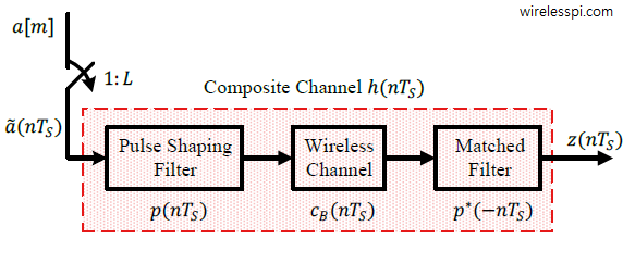
In this article, the modulation symbols are denoted by $a[m]$ while the channel response is represented as $h[m]$, where $m$ is the symbol index. A block diagram of such a structure is drawn in the figure below that shows a composite channel consisting of a pulse shaping filter, a baseband channel and a matched filter.

While the receiver input is denoted by $z(nT_S)$ where $1/T_S$ is the sample rate, the model for a symbol-spaced signal at 1 sample/symbol can be obtained by downsampling the above relation.
\begin{equation}\label{eqEqualizationTMchannelOut}
z[m] = a[m] * h[m]
\end{equation}
In summary, the receiver input is a convolution between the data symbols $a[m]$ and channel taps $h[m]$ taken at symbol intervals (for simplicity, we ignore the effect of a noise whitening filter).
Correlation
The first idea to estimate the channel comes from the definition of an impulse response: the response to an impulse. Ideally, the channel can be learned by sending a single impulse and observe the Rx signal. An impulse, however, has an infinite bandwidth resulting in high sample rates and power consumption even when approximated. Furthermore, a channel estimate based on a single impulse contains significant noise. Therefore, we turn towards some more practical approaches.
For a symbol spaced channel, one of the most straightforward ways to estimate the channel coefficients is to correlate the Rx signal with a known training sequence $a[m]$ of length $N_P$, commonly known as a Pseudo-Noise (PN) sequence. The expression pseudo-noise refers to the fact that the sequence is completely deterministic but possesses noise like autocorrelation properties. The quality of the channel estimate from here depends on the careful design of the training sequence. Ideally, we want to employ a sequence such that its autocorrelation closely resembles an impulse, i.e., it is zero for every shift $i_0 \neq 0$ and a sharp peak for $i_0=0$.
\begin{equation*}
a[m] * a^*[-m] \approx \delta [m]
\end{equation*}
When this sequence is employed as a Tx signal for the correlation operation with a stored copy at the Rx, the output is zero for each shift $i_0$ for a noiseless case. However, when the shift $i_0$ attains a value such that the training sequence embedded in the Tx signal gets aligned with the stored training sequence at the Rx, we observe a sharp peak in the correlation output. From here, the channel impulse response can be obtained as follows.
From Eq (\ref{eqEqualizationTMchannelOut}), the signal $z[m]$ is the training sequence $a[m]$ convolved with the channel impulse response $h[m]$ which is assumed to be a frequency selective channel with length $N_Pap+1$ here.
\begin{equation*}
z[m] = h[m] * a[m]
\end{equation*}
Employing the definition of correlation for complex signals which is the same as convolution with a flipped signal, we can write the correlation output as
\begin{equation*}
z[m] * a^*[-m] = \sum \limits _{i = i_0} ^{i_0+N_P-1} z[i] a^*[i-m]
\end{equation*}
where the index $i_0$ indicates the first sample of the Rx signal used in the correlation. At the instant when the embedded training sequence in the Rx signal and the stored training sequence at the Rx align, we have
\begin{equation*}
\hat h[m] = h[m] * \underbrace{a[m] * a^*[-m]}_{\approx \delta[m]} \approx h[m]
\end{equation*}
i.e., the correlation output sequence is an estimate of the channel. The estimation error is directly proportional to the number of significant taps.
Next, we turn towards a core statistical technique, namely the least squares, to estimate the channel.
Least Squares
Another method to estimate the channel coefficients is the well known Least Squares (LS) technique. This is probably the oldest statistical signal processing technique employed in all kinds of scientific fields, dating back to its discovery by Legendre and Gauss in early 1800s. To keep the discussion simple, we will work with the following assumptions.
- The channel is flat fading, i.e., it is a single tap channel $h[m]$.
\begin{equation*}
z[m] = a[m] \cdot h[m]
\end{equation*}For a channel with multiple taps, i.e., a frequency selective channel, the derivation remains parallel to the one below but matrix operations from linear algebra need to be carried out.
- The channel tap $h[m]$ and the modulated symbols $a[m]$ are real to avoid complex differentiations.
In this setup, the error between the Rx signal $z[m]$ and its actual value $a[m]\cdot h[m]$ is given by
\begin{equation*}
e[m] = z[m] – h[m]\cdot a[m]
\end{equation*}
The error can be both positive or negative, so we want to minimize the magnitude squared value of $e[m]$.
\begin{equation*}
|e[m]|^2 = \Big| z[m] – h[m]\cdot a[m] \Big|^2
\end{equation*}
The derivative of $|e[m]|^2$ with respect to the channel tap $h[m]$ is
\begin{equation}\label{eqEqualizationSquaredErrorDerChannel}
\frac{d}{dh[m]}|e[m]|^2 = 2 e[m]\cdot \overset{\centerdot}{e} [m]
\end{equation}
Utilizing the definition of $e[m]$, its derivative $\overset{\centerdot}{e}[m]$ can be calculated as
\begin{equation*}
\overset{\centerdot}{e}[m] = \frac{d}{dh[m]} \big(z[m] – h[m]\cdot a[m] \big) = -a[m]
\end{equation*}
Plugging it back in Eq (\ref{eqEqualizationSquaredErrorDerChannel}) and equating it to zero yields
\begin{equation*}
2 e[m]\cdot \overset{\centerdot}{e} [m] = -2 \Big(z[m] – h[m]\cdot a[m]\Big)a[m] = 0
\end{equation*}
From here, the estimate $\hat h[m]$ of the channel tap in this flat fading scenario is given by
\begin{equation*}
\hat h[m] = \frac{a[m]z[m]}{|a[m]|^2}
\end{equation*}
For a complex setup, the estimate is given as
\hat h[m] = \frac{a^*[m]z[m]}{|a[m]|^2}
\end{equation}
Multiple pilots symbols can be embedded in the signal to reduce the estimation error through averaging. The above expressions makes sense due to the following two operations being carried out.
- Owing to the underlying correlation technique, multiplication with $a^*[m]$ cancels the phase originating from the modulated symbol within $z[m]$ and leaves only the phase from the channel tap $h[m]$. Utilizing the value of $z[m]$,
\begin{equation*}
a^*[m]z[m] = a^*[m] a[m]h[m] = |a[m]|^2 h[m]
\end{equation*} - Division by $|a[m]|^2$ normalizes the modulation induced magnitude above.
\begin{equation*}
\frac{a^*[m]z[m]}{|a[m]|^2} = \frac{|a[m]|^2h[m]}{|a[m]|^2} = h[m]
\end{equation*}
As mentioned above, the same technique can be applied to a frequency selective channel in the context of matrix operations.
Finally, for a time-varying channel, we begin with the observation that the index $m$ signifies a changing channel for each symbol in a slow fading scenario, i.e., there is little variation from one symbol to the next. To estimate the channel, pilot symbols can be allocated at uniform intervals on which the fading channel tap can be obtained from the above expression. The values for the intermediate data symbols can then be extracted by applying suitable interpolation techniques.
CHANNEL ESTIMATION IN MOBILE WIRELESS SYSTEMS ( with some modification )