Small-scale fading is a phenomenon that arises due to the unguided nature of the wireless medium. Dramatic variations in signal amplitude occur at the Rx from constructive and destructive interference of multipath components originating from the surrounding environment that give rise to small-scale fading. This is the main challenge for designing efficient high-rate wireless communication systems which spawned an array of research activities in the past 50 years aimed to bring the wireless transmission rates closer to their wire counterparts. The technologies for 5G systems have been chosen with the benefit of experience gained from actual implementations over these years.
Delay Spread
To understand how the channel fading phenomenon arises in a wireless channel, consider a modulated waveform in the figure below that is sent over the air at a particular carrier frequency $F_C$. This signal arrives at the destination after traversing several different routes. The wireless channel is represented in the figure through a set of unit impulses with different amplitudes which come together to form our basic channel impulse response.

- The first of these paths is the direct path with a relative amplitude of $\rho_0=1$ and a relative delay of $\tau_0=0$.
- The second of these paths arrives with an amplitude $\rho_1$ and a delay $\tau_1$ with respect to $\tau_0$.
- There are a total of $N_P$ such paths with relative amplitudes and delays denoted by $\rho_i$ and $\tau_i$, respectively, where $i=0$, $1, \cdots$, $N_P-1$.
- The amplitudes $\rho_i$ are determined through large-scale fading phenomenon discussed before.
- The delay spread $T_{\text{Del}}$ of a wireless channel is roughly defined as the time difference between the first and the last significant path.
\begin{equation}\label{equation-delay-spread}
T_{\text{Del}} = \tau_{(N_P-1)}-\tau_0
\end{equation}
See this article for a visualization of how this spread impacts the signal constellation at the receiver. We now describe the effect of movement in the channel.
Doppler Spread
With the introduction of motion in the channel, interesting things happen due to a phenomenon known as Doppler shift, a concept taught in high school physics. Some people have actually paid 300 dollars to learn this concept from the sirens of the police car approaching behind them for a ticket.
Imagine an unmodulated carrier wave $s(t) = \cos 2\pi F_C t$ impinging on the antenna of a mobile in a parked car as drawn in the figure below. The signal arrives at the Rx $\tau_0$ seconds later when the electromagnetic wave travels a distance of $d_0$ m at a speed of approximately $c=3\times 10^8$ m/s. From the time reference of the Tx, this signal is a delay (a right shift) and can be written as
\begin{equation*}
\rho_0\cos 2\pi F_C (t-\tau_0) = \rho_0\cos 2\pi F_C \left(t-\frac{d_0}{c}\right)
\end{equation*}
where $\tau_0 = d_0/c$.

Now imagine that the car is started and is driven at a constant velocity of $\nu$ m/s directly opposite to the antenna. For all further times $t$, the electromagnetic wave that had to travel $d_0$ m now has to cover a distance of $d_0 + \nu t$.
\begin{align}
\rho_0\cos 2\pi F_C \left(t-\frac{d_0+\nu t}{c}\right) &= \rho_0\cos 2\pi F_C \left(t- \frac{\nu}{c}t – \frac{d_0}{c}\right)\nonumber \\
&= \rho_0\cos 2\pi \Big\{\left(F_C- \frac{\nu}{c}F_C\right)t – F_C\tau_0\Big\}\label{eqEqualizationDopplerMP0}
\end{align}
Some comments are now in order.
- As encountered before, the term $-2\pi F_C\tau_0$ is a constant phase shift that arises due to the delay between the Tx and the Rx.
- The frequency of a signal is the term that appears with variable $t$, except the factor $2\pi$. We conclude that the new frequency of the signal is
\begin{equation*}
F^{\text{new}}_C = F_C – \frac{\nu}{c}F_C
\end{equation*}Consequently, there is a shift in frequency which is known as Doppler shift. Here, the Doppler shift, also commonly known as Doppler frequency $F_D$, is
\begin{equation}\label{equation-doppler-shift}
F_D = -\frac{\nu}{c}F_C
\end{equation} - From the above expression, the Doppler shift depends on the carrier frequency $F_C$: the higher the frequency, the higher the Doppler shift and vice versa.
- The Doppler shift also depends on the velocity of the Rx antenna $\nu$. In fact, rewriting the relation as
\begin{equation*}
\frac{F_D}{F_C} = -\frac{\nu}{c}
\end{equation*}reveals that as a fraction of carrier frequency $F_C$, it is just a ratio of the velocities between the mobile and the electromagnetic wave.
- Recall that the expression $d_0 + \nu t$, i.e., an increasing distance, implies that the car in the above figure started moving away from the Tx antenna at an angle of $\pi$ radians. Therefore, the wave has to travel a larger distance and hence the minus sign with the Doppler shift. We can write the actual shift in frequency as
\begin{equation*}
-\frac{\nu}{c}F_C = \frac{\nu\cos \pi}{c}F_C
\end{equation*}Subsequently, for a general angle $\phi$ with respect to the axis of propagation of the wave, the Doppler shift is written as
\begin{equation}\label{eqEqualizationDopplerFreq2}
F_D = \frac{\nu\cos \phi}{c}F_C = F_{D,max}\cos \phi
\end{equation}In other words, we only take into account the velocity component in the direction of arrival of the wave (many scientists write the relation using $c=F_C\lambda_C$ where $\lambda_C$ is the carrier wavelength, in which case the Doppler shift becomes $F_D = \nu\cos \phi/\lambda_C$.
Channel Gains
To determine an expression for the accumulated multipath effect at the Rx, let us simplify the scenario by considering a sinusoidal wave that is sent over the air without any modulation. We can write it as
\[
s(t) = \cos (2\pi F_C t)
\]
where $F_C$ is the carrier frequency of the electromagnetic wave. Although unrelated to the modulated data, the choice of carrier frequency $F_C$ plays a significant role in determining the overall channel effect, as we see now. Nature adds up all these reflected paths at the Rx antenna. Assuming for a moment that there is no movement in the channel, we can write
\[
\begin{aligned}
r(t) &= \rho_0\cos 2\pi F_C (t-\tau_0) + \rho_1\cos 2\pi F_C (t-\tau_1) + \cdots + \rho_{N_P-1}\cos 2\pi F_C (t-\tau_{N_P-1}) \\
&= \sum_{i=0}^{N_P-1} \rho_i \cos 2\pi F_C (t-\tau_i) \\
\end{aligned}
\]
Using the identity $\cos (A-B) = \cos A \cos B + \sin A \sin B$, we can write the above equation as
\[
r(t) = \sum_{i=0}^{N_P-1} \underbrace{\rho_i \cos 2\pi F_C \tau_i}_{\gamma_{i,I}} \cdot \cos 2\pi F_C t – \sum_{i=0}^{N_P-1} \underbrace{-\rho_i \sin 2\pi F_C \tau_i}_{\gamma_{i,Q}} \cdot \sin 2\pi F_C t
\]
This is the standard representation of an I/Q signal. From the above expression, the coefficients of a complex baseband wireless channel can be described as
$$\begin{equation}
\begin{aligned}
\gamma_{i,I}\: &= \rho_i \cdot \cos 2\pi F_C\tau_i \\
\gamma_{i,Q} &= -\rho_i \cdot \sin 2\pi F_C\tau_i
\end{aligned}
\end{equation}\label{equation-channel-gains}$$
Here, we can see why the wireless channel exhibits a complex response even though the Tx signal is real. Any sinusoidal wave with a non-zero phase can be represented as having both a cosine (horizontal) and sine (vertical) component, see the explanation here. The modulated data travels on a sinusoidal wave which arrives at the Rx through multiple delays. This implies that each wave undergoes a different phase shift. Consequently, a summation of sinusoidal waves with different phase shifts gives rise to a final sinusoidal wave that has both a cosine and a sine component. The above description also shows that the channel response is in general a complex function of frequency and time, even if an inphase only modulation such as BPSK is employed for transmission. Therefore, a BPSK Rx has to employ a $Q$ arm as well to scavenge energy lost from the $I$ arm.
Many readers find it easier to understand these summation patterns by drawing the path amplitudes and phases as vectors and then doing vector addition and subtraction. One such example is shown in the figure below for a relatively mild channel. This is also known as a phasor diagram.

What exactly is the effect of such vector summations on the actual waveform? Let us explore the answer to this question below.
Constructive and Destructive Interference
To see how detrimental this wireless channel is, consider the fact that even a slight change in the environment causes a significant change in the channel response. To understand the reasoning below, recall that $\cos (\theta+2\pi)$ $=$ $\cos \theta$, i.e., a phase change of $2\pi$ implies one full cycle. In a similar manner, a phase change of $\pi$ implies half a cycle.
Constructive Interference
Concentrating on the term $2\pi F_C \tau_i$ in Eq (\ref{equation-channel-gains}), the phase of each path completes a full cycle whenever $F_C\cdot \tau_i$ $=$ $1$. Why? Because whenever $2\pi F_C\tau_i$ changes by $2\pi$, the part $F_C\cdot \tau_i$ changes by 1.
\begin{equation*}
\text{variation in }\tau_i = \frac{1}{F_C} \quad \rightarrow \quad \text{Phase change } = 2\pi
\end{equation*}
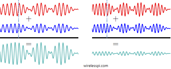
As an example, if the carrier frequency $F_C$ is $1.9$ GHz, $1/F_C = 0.5263$ $ns$ which at the speed of electromagnetic wave $c$ is a distance of $15.8$ cm. In this two-path channel, if the second path length is either of the same length or different by a mere $15.8$ cm, the two waves add constructively to boost the signal amplitude as shown in the left figure below. The vertical line is drawn to identify the similar phases in the two waveforms.

Destructive Interference
On the other hand, assume that the Rx moves a distance such that the phase of each path undergoes a shift of $\pi$ for each $F_C\cdot \tau_i$ $=$ $1/2$.
\begin{equation*}
\text{variation in }\tau_i = \frac{1}{2F_C} \quad \rightarrow \quad \text{Phase change } = \pi
\end{equation*}
In the example above, if the second path length is different by just $7.9$ cm, the two waves add destructively causing the signal amplitude to plummet as shown in the right figure above. The vertical line is drawn to identify the opposite phases in the two waveforms. This happens for a time variation going from $1/F_C$ to $1/2F_C$. Using $c=F_C\cdot \lambda$, this happens from $\lambda/c$ to $(\lambda/2)/c$. We conclude that a displacement of $\lambda/2$ meters is the limit beyond which the channel response changes.
For obvious reasons, most of the actual interference patterns lie in between these two extremes.
Coherence Time and Coherence bandwidth
From the above example, we saw that the channel undergoes a phase shift of $\pi$ over a distance of $\lambda/2$ meters. In other words, if the phase change remains within $\pi$, the channel may be considered time-invariant. This leads to the idea of coherence time $T_C$ as the interval over which the channel response stays nearly constant in time because the wireless device does not go beyond $\lambda/2$ meters. Traveling at a speed of $v$ m/s and using $d = v\cdot t$, this comes out to be
\begin{equation}\label{equation-coherence-time}
T_C = \frac{\lambda}{2v}
\end{equation}
This is an approximation that holds well in empirical observations.
Let us now consider the frequency domain. Since the magnitude response of such a wireless channel also varies with frequency, the range of frequencies over which this magnitude can be assumed approximately constant is termed as Coherence Bandwidth $B_{\text{coh}}$ of the channel.
- From frequency domain characteristics, we have
\[
\underbrace{\delta(t-t_0)}_{\text{Delayed unit impulse}} \stackrel{\mathrm{FT}} {\longleftrightarrow} \underbrace{e^{-j2\pi F t_0 }}_{\text{A Complex sinusoid}}
\]In general, for a signal $x(t)$, we have the time shift property of Fourier Transform as
\begin{equation}\label{equation-time-shift-property}
x(t-t_0)\quad \stackrel{\mathrm{FT}} {\longleftrightarrow}\quad \underbrace{e^{-j2\pi F t_0 }}_{\text{A Complex Sinusoid}}\cdot X(F)
\end{equation}This phase shift being a function of frequency $F$ represents multiplication of the signal spectrum with a complex sinusoid of inverse period $t_0$. The larger this delay $t_0$, the faster the rotation. This is the most important property of Fourier Transform but textbooks have a tendency to mention it as just another property without emphasizing this enough. Thus, we conclude that a signal spread in time causes a faster variation in the spectrum.
- This means that a larger $\tau_i$ produces a faster rotation than a smaller $\tau_i$.
- This in turn results in sharp transitions from high/low to low/high magnitudes in frequency domain.
- Therefore, coherence bandwidth is inversely proportional to the delay spread $T_{\text{Del}}$ (time difference between the first and the last significant path).
\begin{equation}\label{equation-coherence-bandwidth}
B_{\text{coh}} \propto \frac{1}{T_{\text{Del}}} = \frac{1}{\tau_{(N_P-1)}-\tau_0}
\end{equation}
where the definition of delay spread is used from Eq (\ref{equation-delay-spread}).

The coherence bandwidth $B_{\text{coh}}$ for our example channel $C(F)$ in frequency domain is redrawn as shaded regions in the figure above. If we split the channel magnitude response in discrete components, then the portions within a $B_{\text{coh}}$ exhibit a strong magnitude correlation, i.e., their magnitudes attain values near to each other. Two such instances are drawn in the figure as shaded regions.
- When the channel is good, it is good for almost all spectral components within $B_{\text{coh}}$.
- When a deep fade occurs, it drowns almost the complete region within $B_{\text{coh}}$.
Coherence Interval
The ideas of coherence time and coherence bandwidth can be combined into a single factor known as coherence interval which basically is a time-frequency span of $T_C$ seconds over a bandwidth of $B_C$ Hz. The main attraction behind defining a coherence interval is that if the channel does not vary much over $T_C$ seconds and its spectrum does not undergo significant alterations within $B_C$ Hz, then it can be assumed nearly constant on a time-frequency grid without any time or frequency variations.
According to sampling theorem in DSP, the sample rate $1/T_S$ of a signal spanning a bandwidth $B$ Hz should be greater than $2B$ Hz in terms of real samples. For complex samples with both an $I$ and $Q$ parts, this turns out to be
\[
\frac{1}{T_S} \ge B \quad \text{samples/second}
\]
i.e., for a waveform constrained in $B_C$ Hz, we need $B_C$ samples every second. The number of samples collected over an interval of $T_C$ seconds is a coherence interval given by
\begin{equation}
X = B_C \cdot T_C \quad \text{samples}
\end{equation}
This is drawn in the figure below. It is evident that the coherence interval is a time-frequency grid with duration $T_C$ and bandwidth $B_C$.

Let us use the definitions of $T_C$ and $B_C$ to construct an example. For a carrier frequency $F_C=1 GHz$ (i.e., wavelength $\lambda =c/F_C=0.3$ m), walking at a speed of $v=5$ km/hr or $1.39$ m/s yields $T_C$ from Eq (\ref{equation-coherence-time}) as
\[
T_C = \frac{\lambda}{2v} \approx 107 ~\text{ms}
\]
On the other hand, for a displacement of $c(\tau_2-\tau_1)=50$ m between two paths, we write from Eq (\ref{equation-coherence-bandwidth})
\[
B_C = \frac{c}{c(\tau_2-\tau_1)} = 6~\text{MHz}
\]
The coherence interval is now given by
\[
X = T_C\cdot B_C = 642000 ~\text{samples}
\]
This can be a low value for large distances and/or higher carrier frequencies, e.g., at mmWave bands. Next, we turn towards the frequency flat and frequency selective channels.
Frequency Flat Fading
A carrier wave modulated at a low data rate is depicted in the figure below where the first and second multipath are shown above and below the main signal for clarity. Also, the vertical line is drawn to identify the phases in the waveforms at the same point in time.

As plotted before, the phases of these paths might add constructively or destructively or somewhere in between. However, as long as the delay of the second and third paths with respect to the first one is small, the data symbol values of these paths are still (almost) the same and hence there is very low Inter-Symbol Interference (ISI) that shows up on top of those path phases. By ISI, we imply that one symbol does not interfere with the future symbols (e.g., when a path delay is longer than a symbol time). In this sense, the data symbols are all in this together. Depending on the phases of the paths, all the data symbols either experience the same boost or suffer a similar attenuation. The fate of the whole signal is the same.
Before we find the rationale behind the terminology ‘frequency flat’, let us explore the mathematics behind it. The channel impulse response is given by
\begin{equation*}
c(t) = \sum _{i=0}^{N_P -1} \gamma_i \cdot \delta(t-\tau_i)
\end{equation*}
where $\gamma_i$ are channel gains defined in Eq (\ref{equation-channel-gains}), $N_p$ is the number of paths and $\delta(t)$ is the unit impulse signal. When $\tau_i$ are fairly close to each other, the impulses can be taken out as a common factor due to their similarity $\delta(t-\tau_i) \approx \delta(t)$.
\begin{equation}\label{equation-flat-fading-time}
c(t) \approx \sum _{i=0}^{N_P -1} \gamma_i \cdot \delta(t) = h \cdot \delta(t)
\end{equation}
where $h$ is a complex constant expressed as
\begin{equation}\label{equation-flat-fading-gamma}
h = \sum _{i=0}^{N_P -1} \gamma_i
\end{equation}
Here, Eq (\ref{equation-flat-fading-time}) reinforces the concept of the whole signal experiencing the same fate decided by $h$. To summarize, as long as the delay spread is a small faction of the symbol time, i.e., the signal is not too far spread in time with respect to signal bandwidth, all such summations give rise to only one channel tap $h$. For a modulation symbol $s$ sent over the air, the received signal $r$ is thus given by
\[
r = s\cdot h + \text{noise}
\]
This is the model mostly followed in most infrastructure based wireless systems. A simple block diagram of such a setup is drawn in the figure below.

To view this concept in frequency domain, start with a small delay spread, i.e., the signal copies are arriving close to each other at the Rx. Clearly, when the delays $\tau_i$ are small, the rotation periods of frequency domain complex sinusoids in Eq (\ref{equation-time-shift-property}) are large (because the period in frequency domain is given by $1/t_0$ in that equation, just like the period in a time domain sinusoid is $1/F_0$). Not much rotation occurs across the signal bandwidth thus leading to a relatively flat gain. We say that the channel reduces to almost a single complex constant.
A frequency flat fading scenario is drawn in the figure below as an example. Notice that the whole signal bandwidth almost fits within the coherence bandwidth of the channel. Hence, the Rx magnitude depends on the multiplication between the full signal spectrum and (almost) a single attenuation factor shown as a blue dot at $F_C$. This is why it is known as frequency flat fading. Clearly, this blue dot representing the channel attenuation is nothing but $C(F_C)$.

To see how detrimental the effect of fading is on the average bit error probability of digital modulation schemes, consider a wireless channel with no fading and only Additive White Gaussian Noise (AWGN) as the disturbance. The bit error rate is then given by
\begin{equation}\label{equation-ber-awgn}
P_b \propto e^{-\text{SNR}}
\end{equation}
Here, the constants appearing before $e$ and SNR in the exponent are omitted for simplicity. This $P_b$ is drawn for a range of SNR in the figure below where an exponential trend quickly drops the error rate even at moderate SNR. For example, the required SNR at $10^{-4}$ is around $8$ dB for an AWGN channel.

Now a flat fading channel is usually modeled as following a Rayleigh distribution. What this means is that channel gain $\gamma$ in Eq (\ref{equation-flat-fading-gamma}) is a complex Gaussian random variable (whose magnitude is Rayleigh distributed and phase is uniformly distributed between $0$ and $2\pi$). In this case, the bit error rate is only inversely proportional to the SNR.
\begin{equation}\label{equation-ber-rayleigh}
P_b \propto \frac{1}{\text{SNR}}
\end{equation}
This trend is also drawn in the figure above for a comparison with the AWGN channel. It is clear that the bit error rate is much worse here due to the inability of the inverse relationship to bring the error rate down quickly enough. As an example, the required SNR at $10^{-4}$ is around $34$ dB for a fading channel — approximately $26$ dB difference from an AWGN channel!
Next, we explore the topic of frequency selective fading.
Frequency Selective Fading
A carrier wave modulated at a high data rate is depicted in the figure below where the first and second multipath are shown above and below the main signal for clarity. The phases of these paths might add constructively or destructively or somewhere in between. Moreover, due to the long delay of the second and third paths with respect to the first one, the data symbol values of these paths adding up at random instants generate a tremendous amount of Inter-Symbol Interference (ISI) that shows up on top of those path phases. This happens because the random data symbols get summed up into other symbols long after they were actually transmitted. In this sense, there are two phenomenon, and not one, that contribute towards the constructive and destructive interference:
- path delays, and
- symbol values

As before, recognizing the frequency selective fading is a straightforward task in frequency domain. The spectra of all incoming signal paths are the same but different delays in time give rise to complex sinusoids with different inverse periods, see Eq (\ref{equation-time-shift-property}). When these inverse periods are large (due to long time delays), a faster rotation occurs across the signal bandwidth thus leading to spectral selectivity. We conclude that a larger delay spread implies increased frequency selectivity and a smaller coherence bandwidth.
A frequency selective fading scenario is drawn in the figure below as an example where the shaded box represents the coherence bandwidth $B_{\text{coh}}$. Notice that due to the high data rate and hence large signal bandwidth, the whole bandwidth extends beyond the coherence bandwidth of the channel and the Rx magnitude is distributed across a wide spectral region. This is not necessarily bad. As the term selectivity implies, when some part of the signal spectrum is in a deep fade, the rest of the portion is not and hence we are able to achieve frequency diversity through this selective behaviour if we employ an equalizer at the Rx such as Least Mean Square (LMS) or Decision Feedback Equalization (DFE).

Similar to frequency flat and frequency selective channels, there are also time flat (slow) fading and time selective (fast) fading wireless channels for which specific techniques need to be employed. You can learn about them in significant details here.

This post does a fantastic job explaining small-scale fading in wireless channels! The illustrations really helped me grasp the concept better. I appreciate how you broke down the technical aspects into understandable terms. Looking forward to more posts like this!
This post on small-scale fading is incredibly insightful! I appreciate how you broke down the concepts and provided real-world examples. It really helps in understanding the challenges faced in wireless communication. Looking forward to more detailed discussions on improving signal quality!
Great post! I really appreciated the clear explanation of small-scale fading and its impact on wireless communication. The diagrams helped visualize the concepts too. Looking forward to more in-depth discussions on related topics!
Great post! I really appreciated the detailed explanation of small-scale fading and its implications for wireless communication. It’s fascinating how these principles affect everyday connectivity. Looking forward to more insights on wireless technologies!
Great explanation of small-scale fading! I found the examples particularly helpful in understanding how it affects wireless communication. Looking forward to more in-depth posts on the topic!
Great insights on small-scale fading! I appreciate how you explained the impact of multipath propagation on signal quality. It’s fascinating to see how these concepts apply to real-world wireless communication systems. Looking forward to more posts on signal processing!
This post provides a clear and concise explanation of small-scale fading and its impact on wireless communication. I appreciate the inclusion of real-world examples to illustrate the concepts. It really helped me understand how various factors affect signal quality. Looking forward to more posts on this topic!