Costas loop is a carrier phase synchronization solution devised by John Costas at General Electric Company in 1956 [1]. It had an enormous impact on modem signal processing in general and carrier synchronization in particular. At that time, it was customary to send a pilot tone for carrier synchronization along with the data signal which consumed a significant amount of power. Costas was one of the earliest scientists to demonstrate that the carrier phase could be reliably recovered from the Rx signal without the need of a pilot tone. In words of Costas,
"It is unfortunate that many engineers tend to avoid phase locked systems. It is true that a certain amount of stability is a prerequisite but it has been determined by experiment that for this application that stability requirements of single-side band voice are more than adequate. Once a certain degree of stability is obtained, the step to phase lock is a simple one."
Since the publication of his paper, numerous quadrature carrier synchronization loop structures have been developed but their overall structure can easily be traced back to the original work by Costas.
The main theme of these articles is to focus on discrete-time techniques for synchronization. For this purpose, we will follow a continuous-time development due to two reasons.
- Although we deal with its digital implementations now, the Costas loop was originally a pure analog solution and an extensive literature based on continuous-time processing is available. With a similar treatment here, the reader can connect the concepts with that original work.
- Once we treat the Costas loop in continuous-time, we will connect it with a discrete-time implementation for phase synchronization for BPSK and QPSK modulations.
BPSK Modulation
We start with the continuous-time version $v_I(t)$ of the sampled baseband signal $v_I(nT_S)$ given by
\begin{equation*}
v_I(t) = \sum _{i} a_I[i] p(t-iT_M)
\end{equation*}
where
- $a_I[i]$ is the $i^{th}$ data symbol (for example, from a BPSK or QPSK modulation scheme),
- $p(t)$ denotes a transmit pulse, and
- $T_M$ is the symbol time.
The passband signal $r(t)$ is this baseband signal upconverted by a carrier wave with a phase offset of $\theta_\Delta$.
\begin{equation*}
r(t) = v_I(t) \sqrt{2}\cos \left (2\pi F_Ct+\theta_\Delta \right)
\end{equation*}
At the Rx, it is treated in $I$ and $Q$ arms by the sinusoids produced by a Voltage Controlled Oscillator (VCO) with $\hat \theta_\Delta$ as its phase reference. Referring to the terms in figure below,
\begin{equation*}
\begin{aligned}
x_I(t) &= r(t) \cdot \sqrt{2}\cos \left(2\pi F_Ct+\hat \theta_\Delta \right) \\
&= v_I(t) \sqrt{2}\cos \left(2\pi F_Ct + \theta_\Delta\right) \sqrt{2}\cos \left(2\pi F_Ct+\hat \theta_\Delta\right)
\end{aligned}
\end{equation*}

Using the identity $\cos A\cdot \cos B$ $=$ $0.5$ $\{ \cos(A-B)$ $+$ $\cos(A+B) \}$,
\begin{equation*}
x_I(t) = v_I(t) \cos\theta_{\Delta:e} + \underbrace{\cos \left(2\pi 2F_Ct + \theta_\Delta+\hat \theta_\Delta\right)}_{\text{Double frequency term}}
\end{equation*}
where $\theta_{\Delta:e} = \theta_\Delta – \hat \theta_\Delta$ is the carrier phase error. The double frequency term is removed by the lowpass filter in the $I$ arm. We write its output as
\begin{equation*}
z_I(t) = v_I(t)\cos\theta_{\Delta:e}
\end{equation*}
Notice that the quadrature carrier here has a positive sign in the figure above instead of the usual negative sign we encountered in discrete-time phase synchronization loops for complex signal processing. Following a similar line of reasoning and using $\cos A\cdot \sin B$ $=$ $0.5$ $\{\sin(A+B)$ $-$ $\sin(A-B)\}$, the quadrature part of the downconverted and lowpass filtered signal is
\begin{equation*}
z_Q(t) = -v_I(t) \sin\theta_{\Delta:e}
\end{equation*}
The negative sign appears due to using a positive sign at the quadrature carrier. Ignoring the hard limiting operation in the figure above for now and multiplying the two expressions above generates the continuous-time error signal.
\begin{equation}\label{eqPhaseSyncCostasError}
e_D(t) = -v_I^2(t) \cos \theta_{\Delta:e} \sin \theta_{\Delta:e} = – \frac{1}{2} v_I^2(t) \sin 2\theta_{\Delta:e}
\end{equation}
where we have used the identity $\cos A \sin A$ $=$ $0.5\sin 2A$. Clearly, as long as $v_I^2(t)$ varies slowly, the mean curve has a sinusoidal shape which establishes a stable locking point around $\theta_{\Delta:e}=0$.
For the purpose of understanding the operation of the Costas loop, assume for the moment the following.
- The Costas loop is reasonably close to the lock point, i.e., $\theta_{\Delta:e}$ is small. Then, the signal on the $I$ rail after lowpass filtering is close to symbol value $a_I[m]$ at the right time due to $\cos \theta_{\Delta:e} \approx 1$ while that on the $Q$ rail would be close to $\theta_{\Delta:e}$ due to $\sin \theta_{\Delta:e} \approx \theta_{\Delta:e}$.
- The pulse shape is a simple rectangle so that a symbol does not interfere with the neighbouring symbols, hence within a symbol duration
\begin{equation*}
v_I^2(t) \approx a_I^2[m] = (\pm 1)^2 = 1,
\end{equation*}
Consequently, the phase error $\theta_{\Delta:e}$ in Eq (\ref{eqPhaseSyncCostasError}) can be written as
\begin{equation*}
e_D(t) \approx -\frac{1}{2} (2\theta_{\Delta:e}) = -\theta_{\Delta:e}
\end{equation*}
The negative sign in the error term above is catered for by either removing the negative sign before the VCO input, or interchanging the cosine and sine outputs of the VCO and treating the output of the sine as the $I$ arm (this is the solution adopted in conventional Costas loop structures).
Finally, in another version of the Costas loop, the hard limiting operation in the block diagram rejects the small variations usually induced by the signal in the opposite arm and the noise, without affecting a sinusoidal mean curve.
Having obtained this sinusoidal error term, the operation of a Costas loop pretty much mimics a standard Phase Locked Loop (PLL). Due to the $\sin(\cdot)$ term in the phase error detector, the $Q$ rail output is of the same polarity as the $I$ output for one direction of phase difference and opposite polarity for the other direction. Moreover, the sign of the $I$ arm can be taken for making a symbol decision as well. Hence, this phase synchronization circuit provides data estimates as well which was a fundamental shift from the communication circuits of that time.
It has been shown that the performance of the Costas loop is similar to a squaring PLL. The advantage is that the signal processing operations performed through analog circuitry were required only at the carrier frequency here, instead of twice the carrier frequency as in the latter case thus leading to a simpler circuit design.
QPSK Modulation
After understanding the operation of Costas loop for BPSK modulation, it is not difficult to extend its capability to a QPSK case. The Costas loop for QPSK phase synchronization is illustrated in the figure below.

We start with the Rx signal $r(t)$ which includes the carrier wave with a phase offset of $\theta_\Delta$ and a positive sign with the quadrature carrier.
\begin{equation*}
r(t) = v_I(t) \sqrt{2}\cos \left (2\pi F_Ct+\theta_\Delta \right) + v_Q(t)\sqrt{2}\sin \left (2\pi F_Ct+\theta_\Delta \right)
\end{equation*}
At the Rx, it is treated in $I$ and $Q$ arms by the sinusoids produced by a Voltage Controlled Oscillator (VCO) with $\hat \theta_\Delta$ as its phase reference. Referring to the terms in the figure above,
\begin{equation*}
\begin{aligned}
x_I(t) &= r(t) \cdot \sqrt{2}\cos \left(2\pi F_Ct+\hat \theta_\Delta \right) \\
&= \Big\{ v_I(t) \sqrt{2}\cos \left (2\pi F_Ct+\theta_\Delta \right) + \\
&\hspace{1in}v_Q(t)\sqrt{2}\sin \left (2\pi F_Ct+\theta_\Delta \right)\Big\} \sqrt{2}\cos \left(2\pi F_Ct+\hat \theta_\Delta\right)
\end{aligned}
\end{equation*}
Using the identities $\cos A\cdot \cos B$ $=$ $0.5$ $\{ \cos(A-B)$ $+$ $\cos(A+B) \}$ and $\sin A\cdot \cos B$ $=$ $0.5$ $\{\sin(A+B)$ $+$ $\sin(A-B)\}$,
\begin{equation*}
\begin{aligned}
x_I(t) = v_I(t) \cos\theta_{\Delta:e} + v_Q(t) \sin \theta_{\Delta:e} + \text{Double frequency terms}
\end{aligned}
\end{equation*}
where $\theta_{\Delta:e} = \theta_\Delta – \hat \theta_\Delta$ is the carrier phase error. The double frequency terms are removed by the lowpass filter in the $I$ arm. We write its output as
\begin{equation*}
\begin{aligned}
z_I(t) = v_I(t) \cos\theta_{\Delta:e} + v_Q(t) \sin \theta_{\Delta:e}
\end{aligned}
\end{equation*}
Following a similar line of reasoning, the quadrature part of the downconverted signal is
\begin{equation*}
\begin{aligned}
x_Q(t) &= r(t) \cdot \sqrt{2}\sin \left(2\pi F_Ct+\hat \theta_\Delta \right) \\
&= \Big\{ v_I(t) \sqrt{2}\cos \left (2\pi F_Ct+\theta_\Delta \right) + \\
&\hspace{1in}v_Q(t)\sqrt{2}\sin \left (2\pi F_Ct+\theta_\Delta \right)\Big\} \sqrt{2}\sin \left(2\pi F_Ct+\hat \theta_\Delta\right)
\end{aligned}
\end{equation*}
Using the identities $\cos A\cdot \sin B$ $=$ $0.5$ $\{ \sin(A+B)$ $-$ $\sin(A-B) \}$ and $\sin A\cdot \sin B$ $=$ $0.5$ $\{\cos(A-B)$ $-$ $\cos(A+B)\}$,
\begin{equation*}
\begin{aligned}
x_Q(t) = -v_I(t) \sin\theta_{\Delta:e} + v_Q(t) \cos \theta_{\Delta:e} + \text{Double frequency terms}
\end{aligned}
\end{equation*}
The double frequency terms are removed by the lowpass filter in the $Q$ arm. We write its output as
\begin{equation*}
\begin{aligned}
z_Q(t) &= -v_I(t) \sin\theta_{\Delta:e} + v_Q(t) \cos \theta_{\Delta:e}
\end{aligned}
\end{equation*}
Again assuming a rectangular pulse shape and a small phase difference (which implies $\cos \theta_{\Delta:e} \approx 1$ and $\sin \theta_{\Delta:e} \approx 0$), the $I$ signal $v_I(t)$ is close to the symbol value $a_I[m]$ at the right time. Taking its sign is thus approximated as $\hat a_I[m]$. Similarly, the sign of the signal on the $Q$ rail, $v_Q(t)$, is approximately $\hat a_Q[m]$.
\begin{equation*}
\text{sign}\{z_I(t) \} \approx \hat a_I[m], \qquad \text{sign}\{z_Q(t)\}\approx \hat a_Q[m]
\end{equation*}
The purpose of these sign operations is to reject the small variations usually induced by the signal in the opposite arm and the noise. Therefore, the error term from the block diagram above can be given as
\begin{align*}
e_D(t) &= \text{sign}\{z_Q(t)\} z_I(t) – \text{sign}\{z_I(t)\} z_Q(t) \\
&\approx \hat a_Q[m] z_I(t) – \hat a_I[m] z_Q(t)
\end{align*}
While not covered in this article, the expression for a maximum likelihood phase error detector can be simplified as
\begin{equation*}
e_D[m] = \hat a_I[m] z_Q(t) – \hat a_Q[m] z_I(t)
\end{equation*}
where the difference of a negative sign occurs due to the positive sign of the quadrature carrier in this case.
- This comparison shows that the Costas loop can be thought of an approximate solution to the maximum correlation or maximum likelihood technique. Due to this reason, the S-curve of the Costas loop is very similar to the S-curve of the cross product phase error detector in a decision-directed QPSK scenario with a $\pi/2$ phase ambiguity. This phase ambiguity can be resolved through unique words or differential encoding and decoding.
- Other techniques to acquire phase are also available, e.g., the popular M-th power synchronizer in both feedback and feedforward settings.
GNU Radio
In GNU Radio, a Costas loop block is available with the following parameters.
- Loop Bandwidth: The loop bandwidth is the equivalent noise bandwidth of a PLL described earlier and should be adjusted accordingly.
- Order: The loop order depends on the modulation scheme: $2$ for BPSK, $4$ for QPSK and $8$ for $8$-PSK.
- Use SNR: An estimate of SNR before forming the product helps in more accurate phase estimates when a $\tanh(\cdot)$ function is also employed instead of slicing the filter output (i.e., mapping it to the constellation point). This comes from maximum likelihood theory from which the roles played by the SNR estimate and $\tanh(\cdot)$ are derived.
At the time of this writing, there is a slight misrepresentation of the Costas loop in the following statement of the GNU Radio documentation: "The Costas loop locks to the center frequency of a signal and downconverts it to baseband". While this was true for an analog implementation of old days, the digital implementation works at baseband to cater for a phase offset and any residual (fine) frequency offsets.
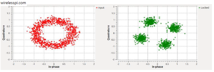
For a loop bandwidth of $2\pi/100$, QPSK modulation and a normalized carrier frequency offset of $-0.043$, the figure below shows the convergence of the loop. The output is rotated because the frequency offset is at the edge of its lock range.

References
[1] Costas, John P. (1956). "Synchronous communications". Proceedings of the IRE. 44 (12): 1713–1718
Thinking purely about the fact that BPSK/QPSK is modulating the phase of the carrier. How can be made sure that the PLL does not remove both LO phase differences AND data-induced phase modulation.
PLL does remove the data-induced phase modulation. However, it is only a sub-block in a digital communication system. It corrects the LO phase difference in the actual signal that now has the LO phase difference removed but modulation intact, presenting its output to a decision device for symbol detection.
Thank you for your answer. I think I was not clear in my question. My understanding is that the Costas Loop should lock on the carrier including its phase offset and frequency offset wrt. the receiver carrier. But the loop cannot distinguish between data induced phase offset and hardware LO induced phased offset. Is that resolved by the squaring operation which effectively removes the data-induced phase modulation?
Yes that is correct. In fact, that’s exactly the principle of operation of a PLL.
If using a Costas Loop for phase synchronisation prior to BPSK demodulation, is phase ambiguity still an issue? Intuitively, I would say no since the loop can be used to ideally remove any phase perturbations from the carrier. Maybe you could clarify this. Thank you!
Yes phase ambiguity is an still issue because the Costas Loop cannot differentiate between two possible phases of a BPSK signal. Taking the sign of the target cannot differentiate between phase $0$ and phase $\pi$.
Thanks for the article. I have often seen BPSK Costas loop error derived from I*Q but you have sliced I then multiplied by Q. Is that an option or a must?
I times Q would be a non-data-aided version of the phase error detector. Sliced I times Q is a decision-directed version of the same. This works better for good SNR conditions since the noise is removed at each iteration, and probably what the original inventor Costas intended to achieve.
Thanks, makes sense.
Hello. Great article. Do you know where I can find a python or C implementation of the Costas loop ? (similar to the one from the PLL article)
You can slightly modify the PLL code for a Costas loop implementation. Or search for GNU Radio Costas loop block and find its C++ code.
Thanks for the tip 😀