The LMS algorithm was first proposed by Bernard Widrow (a professor at Stanford University) and his PhD student Ted Hoff (the architect of the first microprocessor) in the 1960s. Due to its simplicity and robustness, it has been the most widely used adaptive filtering algorithm in real applications. An LMS equalizer in communication system design is just one of those beautiful examples and its other applications include noise and echo cancellation, beamforming, neural networks and so on.
Background
The wireless channel is a source of severe distortion in the received (Rx) signal and our main task is to remove the resulting Inter-Symbol Interference (ISI) from the Rx samples. Equalization refers to any signal processing technique in general and filtering in particular that is designed to eliminate or reduce this ISI before symbol detection. In essence, the output of an equalizer should be a Nyquist pulse for a single symbol case. A conceptual block diagram of the equalization process is shown in the figure below where the composite channel includes the effects of Tx/Rx filters and the multipath.

A classification of equalization algorithms was described in an earlier article. Here, we start with the motivation to develop an automatic equalizer with self-adjusting taps.
Motivation
A few reasons for an adaptive equalizer are as follows.
Channel state information
In developing the coefficients for an equalizer, we usually assume that perfect channel information is available at the Rx. While this information, commonly known as Channel State Information (CSI), can be gained from a training sequence embedded in the Rx signal, the channel characteristics are unknown in many other situations. In any case, the quality of the channel estimation is only as good as the channel itself. As the wireless channel deteriorates, so does the reliability on its estimate.
Time variation
Even when the wireless channel is known to a reasonably accurate level, it eventually changes after some time. We saw in detail how time variations in the channel unfold on the scale of the coherence time and how this impacts the Rx signal. For that reason, an equalizer needs to automatically adjust its coefficients in response to the channel variations. Nature favours those who adapt.
Utilization of available information
In situations where the channel is estimated from a training sequence and a fixed equalizer is employed, it is difficult to incorporate further information obtained from the data symbols. For an adaptive equalizer, the taps can be adjusted first from the training sequence and then easily driven through the data symbols out of the detector in a decision-directed manner in real time.
We next develop an intuitive understanding of its operation.
An Intuitive Understanding
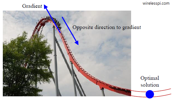
Before we discuss the LMS algorithm, let us understand this concept through an analogy that appeals to intuition. For what follows, a gradient is just a mere generalization of the derivative (slope of the tangent to a curve) for a multi-variable function. We need a multi-variable derivative’ (i.e., a gradient) in our case because the equalizer has multiple taps, all of which need to be optimized.
Assume that you are on a holiday with your family and spending the day in a nice theme park. You are going upwards on a roller coaster and hence the gradient is in the upward direction as shown in the figure below. Also assume that you are sitting in the front seat, have access to a (hypothetical) set of brakes installed and there is no anti-rollback mechanism which prevents the coasters from sliding down the hill.

Suddenly the electricity in the park goes out. Leaving the roller coaster to slide all the way down the hill would be catastrophic, so your strategy is to
- first apply the brakes preventing the sudden and rapid drop,
- leave the brakes to slightly descend in the direction opposite to the gradient,
- apply the brakes again, and
- repeat this process.
Repeating the above steps in an iterative manner, you will safely reach the equilibrium point. With this intuition in place, we can discuss the LMS algorithm next.
The LMS Algorithm
Refer to the top figure in this article and assume that the relevant parameters have the following notations.
- The $m$-th data symbol is denoted by $a[m]$ that represents an amplitude modulated system.
- The corresponding matched filter output is written as $z[m]$.
- The equalizer coefficients are given by $q[m]$.
- The equalizer output is the signal $y[m]$.
- The error signal at this moment is denoted by $e[m]$.
We start with a performance function that has a similar valley type shape, e.g., the squared error.
\begin{align*}
~\text{Mean}~ |e[m]|^2 &= ~\text{Mean}~ \left|a[m] – y[m]\right|^2 = ~\text{Mean}~ \left|a[m] – z[m]*q[m]\right|^2\\
&= ~\text{Mean}~ \left|a[m]- \sum _{l=-L_q}^{L_q} q[l]\cdot z[m-l]\right|^2
\end{align*}
The figure on the left below draws this quadratic curve as a function of one equalizer tap $q_0[m]$ which is similar to the roller coaster analogy we saw before. On the same note, the right figure draws the same relationship as a quadratic surface of two equalizer taps, $q_0[m]$ and $q_1[m]$ where a unique minimum point can be identified. Extending the same concept further, Mean $|e[m]|^2$ can be dealt with as a function of $2L_q+1$ equalizer taps $q_l[m]$ and a unique minimum point can be reached. It is unfortunate that we cannot graphically draw the same relationship for a higher number of taps.

We can start at any point on this Mean $|e[m]|^2$ curve and take a small step in a direction where the decrease in the squared error is the fastest, thus proceeding as follows.
- If the equalizer taps $q[m]$ were constant, we could use the symbol time index $m$ for the equalizer tap $q[m]$ (because we are treating it as a discrete-time sequence). But our equalizer taps are changing with each symbol time, so we need to bring in two indices, $m$ for time and $l$ for the equalizer tap number which we assign as a subscript. Each tap for $l=-L_q$, $\cdots$, $L_q$ is updated at symbol time $m+1$ according to
\begin{equation*}
q_l[m+1] = q_l[m] + \text{a small step}
\end{equation*}Here, $q_l[m]$ means the $l^{th}$ equalizer tap at symbol time $m$.
- The fastest reduction in error happens when our direction of update is opposite to the gradient of Mean $|e[m]|^2$ with respect to the equalizer tap weights.
\begin{equation*}
q_l[m+1] = q_l[m] + \text{a small step opposite to the gradient of}~\text{Mean}~ |e[m]|^2
\end{equation*} - The gradient is a mere generalization of the derivative and we bring in a minus sign for moving in its opposite direction.
\begin{equation}\label{eqEqualizationTapUpdate}
q_l[m+1] = q_l[m] – ~\text{Mean}~ \frac{d}{dq_l[m]} |e[m]|^2
\end{equation} - Utilizing the definition of $e[m]$ as
\[
a[m]- y[m]= a[m] – \sum _{l=-L_q}^{L_q} q[l]\cdot z[m-l]
\]the derivative for each $l$ can be written as
\begin{align*}
\frac{d}{dq_l[m]} |e[m]|^2 = -2 e[m]\cdot z[m-l]&~~\\
&\text{for each }l = -L_q,\cdots,L_q
\end{align*}Substituting this value back in Eq (\ref{eqEqualizationTapUpdate}), we can update the set of equalizer taps at each step as
\begin{equation*}
q_l[m+1] = q_l[m] + 2 ~\text{Mean}~ \Big\{e[m]\cdot z[m-l]\Big\}
\end{equation*} - Now let us remove the mean altogether, a justification for which we will shortly see, and get
\begin{equation*}
q_l[m+1] = q_l[m] + 2 e[m]\cdot z[m-l]?
\end{equation*} - The question mark above is there to indicate that we are probably forgetting something. Remember the brakes in the roller coaster analogy? We need to include an effect similar to the brake here, otherwise the effect of the gradient on its own will result in large swings on the updated taps. Let us call this parameter representing the brakes a step size and denote it as $\mu$. We will see the effect of varying $\mu$ below.
$$ \begin{equation}
\begin{aligned}
q_l[m+1] = q_l[m] + 2 \mu &\cdot e[m]\cdot z[m-l]\\
&\text{for each }l = -L_q,\cdots,L_q
\end{aligned}
\end{equation}\label{eqEqualizationLMS}$$
A brilliant trick
In an actual derivation of an optimal filter, it is the statistical expectation of squared error that is minimized, i.e.,
\begin{equation*}
~\text{Mean}~ ~|e[m]|^2
\end{equation*}
and hence the term mean squared error. Now if Widrow and Hoff wanted to derive the adaptive algorithm that minimizes the mean squared error, they needed to obtain the statistical correlations between the Rx matched filtered samples themselves as well as their correlations with the actual data symbols. This is a very difficult task in most practical applications.
So they proposed a completely naive solution for such a specialized problem by removing the statistical expectation altogether, i.e., just employ the squared error $|e[m]|^2$ instead of mean squared error, Mean $|e[m]|^2$. This is what we saw in the algorithm equation derived above. To come up with such a successful workhorse for filter taps adaptation, when everyone else was running after optimal solutions, was a brilliant feat in itself.
It turns out that as long as the step size $\mu$ is chosen sufficiently small, i.e., the brakes are tight enough in our analogy, the LMS algorithm is very stable — even though $|e[m]|^2$ at each single shot is a very coarse estimate of its mean.
The Two Stages
Figure below illustrates a block diagram for implementing an LMS equalizer. The matched filter output $z[m]$ is input to a linear equalizer with coefficients $q_l[m]$ at symbol time $m$. These taps are updated for symbol time $m+1$ by the LMS algorithm that computes the new taps through Eq (\ref{eqEqualizationLMS}). The curved arrow indicates the updated taps being delivered to the equalizer at each new symbol time $m$.

The input to the LMS algorithm is the matched filter output $z[m]$ and error signal $e[m]$. In general, there are two stages of the equalizer operation.
- Training stage: In the training stage, the error signal $e[m]$ is computed through subtracting the equalizer output $y[m]$ from the known training sequence $a[m]$.
- Decision-directed stage: When the training sequence ends, the LMS algorithm uses the symbol decisions $\hat a[m]$ in place of known symbols and continues henceforth.
The three steps performed by an LMS equalizer are summarized in the table below. It is important to know that since the update process continues with the input, the equalizer taps — after converging at the optimal solution given by the MMSE solution — do not stay there. Instead, they just keep hovering around the optimal values (unlike the roller coaster analogy which comes to rest at the end) and add some extra error to the possible optimal solution.

If you are a radio/DSP beginner, you can ignore the next lines. Using $y[m] = z[m] * q_l[m]$ (where * denotes convolution) and applying the multiplication rule of complex numbers $I\cdot I$ $-$ $Q\cdot Q$ and $Q\cdot I$ $+$ $I\cdot Q$, we can see that these are $4$ real convolutions for a complex modulation scheme. While the inphase coefficients $q_{l,I}[m]$ combat the inter-symbol interference in the inphase and quadrature channels, the quadrature coefficients $q_{l,Q}[m]$ battle the cross-talk between the two channels. This cross-talk is usually caused by an asymmetric channel frequency response around the carrier frequency.
On the Step Size $\mu$
To observe the effect of the step size $\mu$ on the performance of the LMS equalizer, we incorporate a $4$-QAM modulated symbols shaped by a Square-Root Raised Cosine pulse with excess bandwidth $\alpha=0.25$. The impulse response of the wireless channel is given by
\[
h[m] = [0.1~0.1~0.67~01.9~-0.02]
\]
and the resulting curves are averaged over 100 simulation runs for a symbol-spaced equalizer. We consider the following three different values of $\mu$.
\begin{equation*}
\mu = 0.01,\quad \mu = 0.04, \quad \mu = 0.1
\end{equation*}
Figure below draws the corresponding curves for all three values of $\mu$, regarding which a few comments are in order.

- A large value of $\mu$ generates an equalizer response that converges faster than that for a smaller value of $\mu$. This makes sense from the form of the equalizer tap update where the new tap at each symbol time $m$ is generated through the addition of $2\mu e[m]z[m-l]$ in the previous tap value. The larger the $\mu$, the larger the update value and hence faster the convergence.
- So why not choose $\mu$ as large as possible? From the roller coaster analogy, it can flip over in any direction if it is thrown towards the equilibrium point too quickly by not properly applying the brakes. Recall that the LMS algorithm, after converging to the minimum error, does not stay there and fluctuates around that value. The difference between this minimum error and the actual error is the excess mean square error. While it is not clear from the figure above, a larger $\mu$ results in a greater excess error and hence there is a tradeoff between faster convergence and a lower error.
- From the update expression $2\mu e[m]z[m-l]$ which dictates how each tap is generated through the previous tap value, we also infer that for a given $\mu$, the convergence behaviour (and stability) of the LMS algorithm also depends on the signal power at the equalizer input. In a variant known as normalized LMS equalizer, this signal power is estimated to normalize $\mu$ at each symbol time $m$.
- For $\mu=0.1$, the corresponding equalizer taps are shown converging to their final values in the figure below. The equalizer takes many hundreds of symbols before approaching the tap values with acceptable $~\text{Mean}~ ~|e[m]|^2$. This is typical of this kind of processing in an iterative fashion.
- The convergence time of the LMS equalizer also depends on the actual channel frequency response. If there is not enough power in a particular spectral region, it becomes difficult for the equalizer to prepare a compensation response. As a result, a spectral null reduces the convergence speed and hence requires a significantly large number of symbols. This had been one of the bottlenecks in the high rate wireless communication systems. This was the motivation behind designing frequency domain equalizers.
- An LMS equalizer is also extensively used in high speed serial links in conjunction with Decision Feedback Equalization (DFE).
- Finally, the process of equalizer taps convergence is more interesting to watch from a constellation point of view as it unfolds in a 3D space for equalizer output $y[m]$, which I called a dynamic scatter plot. If this page was a 3D box and we could go towards one side of the scatter plot, we would have viewed it as in the figure below. Since the equalizer taps are initialized as all zeros, the equalizer output $y[m]$ starts from zero. Then, the four $4$-QAM constellation points trace a similar trajectory taken by $~\text{Mean}~ |e[m]|^2$ and $q_l[m]$ before. The figure has been plotted for $\mu=0.1$. Note that the varying amount of gap between some constellation points arises from the randomness of the data symbols consisting of one out of four possible symbols during each $T_M$.


Accelerating the Convergence
An LMS equalizer has been the workhorse for wireless communication systems throughout the previous decades. However, we saw in the above example that it takes many hundreds or thousands of symbols before the LMS equalizer converges to the optimum tap values. As a general convergence property, remember that the shortest settling time is obtained when the power spectrum of the symbol-spaced equalizer input (that suffers from aliasing due to 1 sample/symbol) is flat and the step size $\mu$ is chosen to be the inverse of the product of the Rx signal power with the number of equalizer coefficients. A smaller step size $\mu$ should be chosen when the variation in this folded spectrum is large that leads to slower convergence.
In the last two decades of the 20th century, there was a significant interest in accelerating its convergence rate. Two of the most widely employed methods are explained below.
Variable step size $\mu$
It is evident that the convergence rate is controlled by the step size $\mu$. Just like we saw in the case of a Phase Locked Loop where the PLL constants are reconfigured on the fly, it makes sense to start the LMS equalizer with a large value of $\mu$ to ensure faster convergence at the expense of significant fluctuation during this process. After converging closer to the optimal solution, it can be reduced in steps such that $\mu$ during the final tracking stage is a small enough value to satisfy the targeted excess mean square error.
Cyclic equalization
Instead of modifying $\mu$, this method focuses on the training sequence that is sent at the start of the transmission to help the Rx determine the synchronization parameters as well as the equalizer taps. It was discovered that if this training sequence is made periodic with the same period as the equalizer length, the taps can be computed almost instantly. This is done through exploiting the periodicity in the stored sequence $a[m]$ and the incoming signal $z[m]$. The periodicity implies that a Discrete Fourier Transform (DFT) of these sequences can be taken and multiplied point-by-point for each DFT index $k$. After normalizing the result for each $k$ by the Rx power in that spectral bin, an inverse Discrete Fourier Transform (iDFT) is taken to determine the equalizer taps $q[m]$ (on a side note, this same method can also be used to estimate the channel impulse response $h[m]$ instead of the equalizer taps and then use another equalizer, such as the maximum likelihood sequence estimation or MMSE equalizer, to remove the channel distortion).
Although cyclic equalization is a very interesting technique, it is largely abandoned in favour of a better alternative for high speed wireless communications, namely the frequency domain equalization.
LMS Variants
In summary, the LMS equalizer has been incorporated into many commercial high speed modems due to its simplicity and coefficients adaptation of a time-varying channel. For further simplification, some of its variations employ only the sign of the error signal or that of the input samples. Three such possible variations for tap adaptation are as follows.
\begin{align*}
q_l[m+1] = q_l[m] + 2 \mu &\cdot \text{sign} (e[m])\cdot z[m-l]\\
&\hspace{1.5in}\text{for each }l = -L_q,\cdots,L_q \\
q_l[m+1] = q_l[m] + 2 \mu &\cdot e[m]\cdot \text{sign}(z[m-l])\\
&\hspace{1.5in}\text{for each }l = -L_q,\cdots,L_q \\
q_l[m+1] = q_l[m] + 2 \mu &\cdot \text{sign}(e[m])\cdot \text{sign}(z[m-l])\\
&\hspace{1.5in}\text{for each }l = -L_q,\cdots,L_q
\end{align*}
It is evident that the last variant is the simplest of all, consisting of just the signs of both quantities. On the downside, it also exhibits the slowest rate of convergence.
Conclusion
LMS algorithm, like other adaptive algorithms, behaves similar to a natural selection phenomenon but the difference is that we cannot afford to generate 100s of variants at each step to find out the best. Instead of iteration, variation and then selection, we select the likely best variant in a serial evolution manner.