Diversity in Wireless Communication Systems

Diversity is one of those few ideas that are extremely dumb and extremely clever at the same time. It can be explained in one sentence as well as in a whole book. The basic idea, nevertheless, is quite simple.

What is Diversity?

Consider the following two different cases.

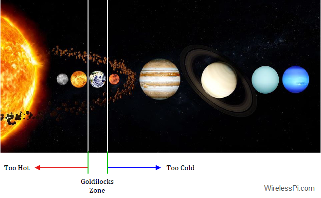
• Many phenomena in the world need a series of outcomes to succeed. For instance, for life to exist in the cold and dark universe, we need a star to provide energy as heat. A planet is also required as a home. Furthermore, this planet must reside in the Goldilocks Zone of that star. Similar to the baby bear’s porridge in the story Goldilocks and the Three Bears, this is the habitable zone around the star where the temperature is just right — neither too hot, nor too cold — for liquid water to exist, see the figure below. This planet must also inhibit several specific elements in the right proportions at the right places. As another example, many vital body organs such as heart and brain must function properly for a person to live. If any of them fails, there is no more life.

  

  Speaking in mathematical terms, we can say that if the requirements A, B, C, etc. in the above examples are all independent to each other, and we denote their probabilities as $P_A$, $P_B$, $P_C$, etc., then the probability of a successful outcome is
  \[
  P(\text{success}) = P_A\cdot P_B \cdot P_C \cdots
  \]
  Clearly, when any single term on the right side becomes zero, the chance of success on the left side becomes zero too. If the probability of all the terms is the same, given by $p$, and there are $L$ such participating factors, then the above equation yields

  \begin{equation}\label{equation-nature}
  P(\text{success}) = p^L
  \end{equation}

  All this comes from the the 2nd law of thermodynamics, according to which the failure cases (disorganized states) should be much higher than the success cases (organized states).

• On the other hand, many other phenomena require a single outcome to succeed. Most people on the planet are born with two kidneys and two lungs. If one of them fails, they can still live a healthy life with some precaution. This is the essence of diversity. Now consider the main active agent in the known world: a human mind. With the ability to make decisions and influence outcomes as well as iterate over the design in a short time span, human designs can be made more resilient than those of nature. Let us take a simple analogy. If you toss a coin, you only have a $50\%$ (i.e., $1/2$) chance of getting a head.
  \[
  \underbrace{\{H\}, \{T\}}_{\text{1 out of 2}}
  \]
  However, if you toss two coins, there is a $75\%$ (i.e., $3/4$) chance that you will have at least 1 head as the outcome.
  \[
  \underbrace{\{H, H\}, \{H, T\}, \{T, H\}, \{T, T\}}_{\text{3 out of 4}}
  \]

  

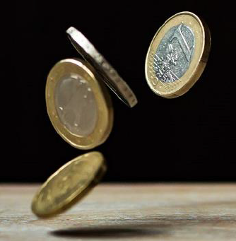
  These odds increase in your favor with more coins. For 4 coins shown in the figure above, there are $2^4$ $=$ $16$ possible outcomes and the probability of at least one of them having a head improves to around $94\%$ (i.e., $15/16$).

In the Context of Wireless Systems

Consider the block diagram of a simple communication system in the figure below that depicts three main blocks involved as well as the wireless channel. Notice that everything is in the hands of the system designer except the wireless channel that depends on large-scale and small-scale fading (as well as all the distortions encountered in the Tx/Rx frontends). These blocks, namely coding + decoding, modulation + demodulation and Tx/Rx frontends, can be optimized with the most ingenious of ideas. Nevertheless, a wireless channel in a bad state can still break the system. This is because when a number (or in our case, a waveform) is multiplied with zero, all we get is a zero without knowing if that number was 7, 16 or 21. This is why the bit error probability for a fading channel is significantly worse than that for the AWGN case.

Diversity implies using two or more statistically independent replicas for the transfer of the same information. This improves the reliability of the received message because nothing can recover the data signal in a deep fade except getting more copies of the same message. Just like the probability of at least one head in coin tosses increases with the number of coins, the probability of at least one copy out of a fade increases with the number of diverse copies. This is shown as the signal traversing multiple routes within the wireless channel in the figure above (as a reminder, this is a different concept than multipath because the term route here can denote a simple retransmission in time or reception from another antenna, for example). As long as any one of these copies enables the signal reception at a sufficient SNR, the system operation is a success. This message replication can be provided in different forms (e.g., time, frequency, polarization, space) but a simple illustration of how combining the same signal from two different antennas improves the signal part is drawn in the figure below.

Coming to the mathematical side, if the probability of each copy being rendered useless by channel fading is $P_A$, $P_B$, $P_C$, and so on, the transmission will only fail if \bbi{each and every one of them} experiences fading at the same time. We can write
\[
P(\text{failure}) = P_A\cdot P_B\cdot P_C \cdots
\]
Extending this idea further, if the probability of an individual fade given by $p$ is the same for all the replicas (a realistic assumption), the probability of overall link failure with $L$ diverse copies is given by
\begin{equation}\label{equation-p-failure}
P(\text{failure}) = p^L
\end{equation}
And the corresponding probability of success is given by

Compare this with Eq (\ref{equation-nature}) and notice how the relation is completely reversed. We conclude that the higher the number of diverse replicas $L$, the lower the chances of a failed transmission. This number $L$ is known as diversity order. This diversity is the fundamental reason behind how cellular networks like 5G have overcome the harsh wireless channel for high speed data transmission. In fact, you can easily extrapolate the idea here to grasp how massive MIMO systems with a large number of antennas (i.e., a large $L$ in the above expression) effectively transform a fading channel into a simple AWGN one.

Effect on BER

Now without proof, we state that the probability $p$ of a deep fade in a Rayleigh fading channel is inversely proportional to the Signal to Noise Ratio (SNR).
\begin{equation}\label{equation-p-snr}
p \approx \frac{1}{SNR}
\end{equation}
where the exact constant that depends on the modulation scheme is ignored for simplicity. Therefore, Eq (\ref{equation-p-failure}) tells us that the probability of failure or Bit Error Rate (BER) is related to SNR as
\begin{equation}\label{equation-ber-snr}
BER~ \propto ~p^L =\frac{1}{SNR^L}
\end{equation}
This is an interesting result revealed by the above expression: an increasing diversity order affects the BER in an exponential fashion! In another article, we will relate this trend to the slope of the BER curve but a figure for selection combining is drawn near the end of this page. While we did not go into fancy derivations proving this result due to the limited mathematical scope of this text, this is a rather neat way of comprehending the role of diversity in a wireless system.

Types of Diversity

The interesting part about diversity is that these multiple copies mentioned above are not simply repeated transmissions. Instead, mathematicians and engineers have devised brilliant strategies in various forms of diversity that are practically employed.

Time Diversity

A wireless channel is changing with time. In the simplest case, a wireless signal can be sent twice over the same channel at two different time instants. The gap between these instants should be slightly longer than the average duration of a fading event. In real world, however, this technique is wasteful of resources available at the disposal of a communication system designer. Therefore, a clever scheme known as Forward Error Correction (FEC) is used instead of simply repeating the original transmission. During the coding process, redundant bits are added to the information bits in a deterministic manner. At the Rx, a decoder runs suitable algorithms to figure out the transmitted bits even when the received signal has suffered from multiple errors. A state-of-the-art coding scheme known as Low Density Parity Check (LDPC) codes has been chosen for 5G data channels.

Interleaving is another form of time diversity. To combat a long series of errors during the same fading event known as burst errors, the information bits are interleaved at the Tx side and de-interleaved at the Rx side. For example, one method of interleaving is to read the bits in rows and write them out in columns so that two adjacent bits in the information stream are actually one column apart at the input of the coder. This prevents the burst from erasing an adjacent set of bits.

Frequency Diversity

The destructive interference at the antenna we mentioned earlier causes a fade in the received power because the phase difference between the two paths is either (close to) $180^\circ$ or a multiple thereof. Clearly, the frequency $F$ sets the number of wavelengths that fit into the length of the transmission path. The fraction left thereafter determines the arriving phase at the Rx. Opposite phases of two such paths cancel the received signal.

Now if we send another copy of the signal at a slightly different frequency, the phase difference between the two paths will not be close to $180^\circ$ as long as the other frequency is more than the coherence bandwidth apart. It just becomes similar to the two coins example we saw above and the probability of phases canceling out for both of these frequencies is low. This gives rise to frequency diversity utilized by wideband signals. When one part of the spectrum is in fade, the other part of the spectrum is not affected and usually provides enough information for signal recovery.

Equalizers in wireless communication systems exploit this frequency diversity to mitigate the channel effect. For instance, an LMS equalizer can track a time varying channel to remove the Inter-Symbol Interference (ISI) and a Decision Feedback Equalizer (DFE) utilizes the detected symbols to erase the impact of the channel distortion. Furthermore, a RAKE receiver is a special kind of equalizer in Code Division Multiple Access (CDMA) systems, the technology behind 3G cellular networks. In 4G and 5G systems, equalization in frequency domain has been adopted due to its superiority over time domain equalization, see the article on OFDM as an example.

Spatial Diversity

When some people first hear the term space, it causes some confusion in regards to what the concept of diversity has to do with space! For clarification purpose, space refers to the diversity provided by another antenna at a different position. The idea is similar to human ears in the form of two receive antennas that help us not only to capture sounds from different locations but also to estimate their directions.

The starting point is the realization that multipath fading cannot take away energy that has already been injected into the air. Since the signal is traveling in time and space, the energy has simply been redistributed in three spatial dimensions. The only problem is the fraction of energy impinging on the Rx antenna where wave summation occurs in a destructive manner. This fraction of energy can be significantly increased by tapping into a different part of space. For example, if there is a second antenna placed at the Rx sufficiently apart from the first antenna, the phase relationship between the two paths would be different over there.

In major cellular and wireless networks of the past, space diversity has been employed with the help of multiple Tx antennas and/or multiple Rx antennas giving rise to Multiple Input Multiple Output (MIMO) systems. The interesting thing about spatial diversity is that signal transmission takes place at the same time over the same frequency band. In comparison, both time and frequency diversity require additional bandwidth, an increasingly scarce resource. The benefits thus provided are worth the material cost of additional antennas, their RF chains and associated signal processing. We explain the idea of space diversity with the help of a simple scheme: Selection Combining (SC).

Consider a wireless link with $1$ Tx antenna and $2$ (or more) Rx antennas as shown in the figure below. At each symbol time, a data symbol $s$ is transmitted which belongs to a Quadrature Amplitude Modulation (QAM) scheme. To focus on the events happening within one symbol time only, we have dropped the time index $m$ from the modulation symbol $s[m]$ here.

• In this setup, $r_1$ is the signal received by the first antenna while $r_2$ is the signal received by the second antenna.
• $h_1$ is the flat fading channel gain between the Tx antenna and the first receive antenna. Remember that there is a difference between channel paths and channel taps. The bandwidth of our signal determines the number of channel taps in our system, regardless of the actual number of channel paths. These taps are usually denoted by $h[n]$ in wireless literature. More details on this can be found in Chapter 8 of my book.
• $h_2$ is the flat fading channel gain between the Tx antenna and the second receive antenna.

In selection combining, the Rx computes the instantaneous signal strength at each of the antennas and selects the one with the highest power. In other words, the branch with the best channel gain $h_i$ is chosen for demodulation. This exploitation of channel knowledge at the Rx provides a significant diversity gain.

To see how the performance is enhanced with selection combining, the average bit error rate is drawn in the figure below for a Rayleigh fading channel with $N_R=1$, $2$ and $3$ Rx antennas where ideal bit error rate for an AWGN channel is also shown. This bit error performance from selection diversity improves with increasing number of antennas. For instance, by adding a second antenna at the Rx at a target bit error rate of $10^{-4}$ depicted by the ellipse, the average SNR requirement in a flat fading scenario drops from around $34$ dB to less than $20$ dB. This is further reduced to less than $15$ dB when a third antenna is also available. We conclude that the improvement is substantial for the first few antennas before the law of diminishing returns flattens the marginal gain from each additional antenna.

One drawback of selection combining is that it discards the useful energy arriving at the other antennas at the expense of simple hardware requirements and computational simplicity. In many situations, such a trade-off is desirable. Otherwise, a better approach known as Maximal Ratio Combining (MRC) can be employed. Finally, spatial diversity can also be converted into time and frequency diversity through appropriate techniques.